Tutorial
This tutorial first gives a general overview of the RAMANMETRIX features, followed by step-by-step instructions covering an example for a classification and regression task.
General overview
Main interface
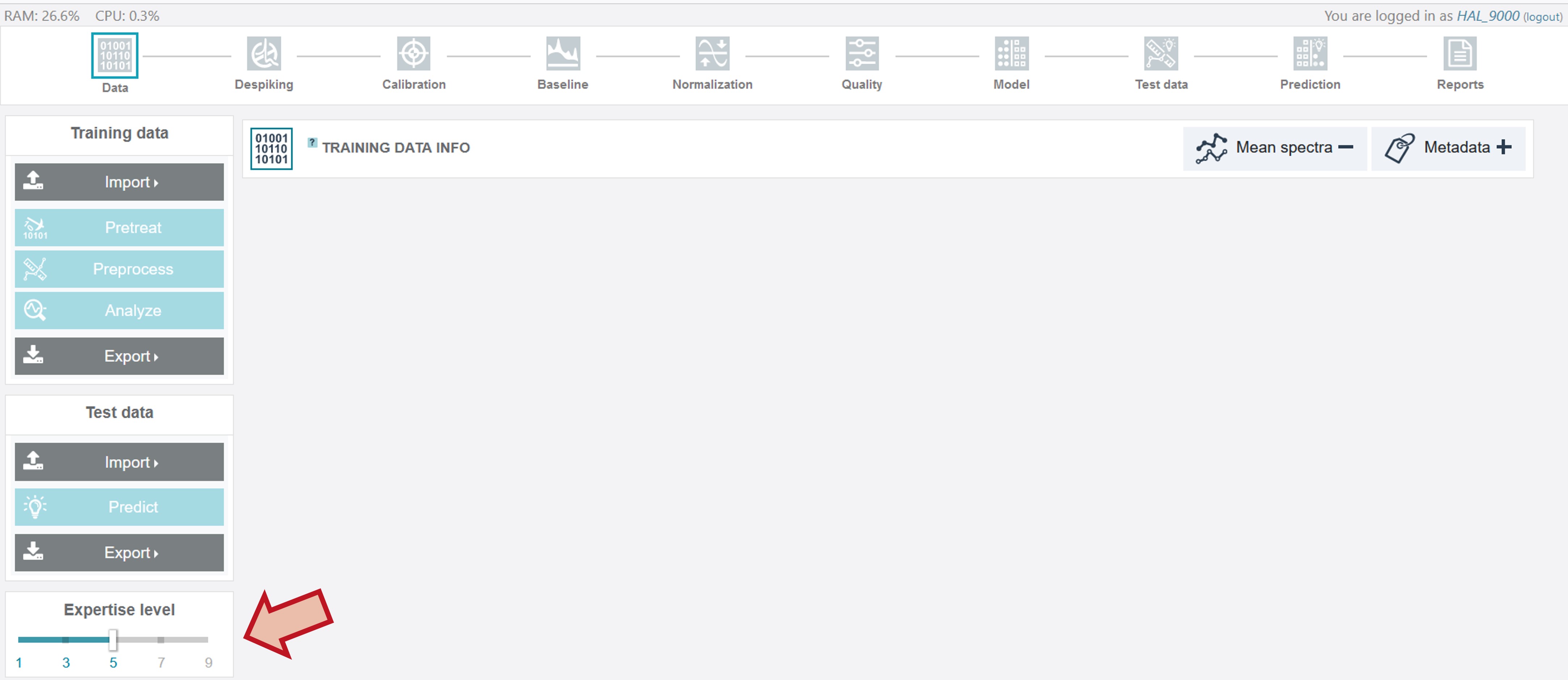
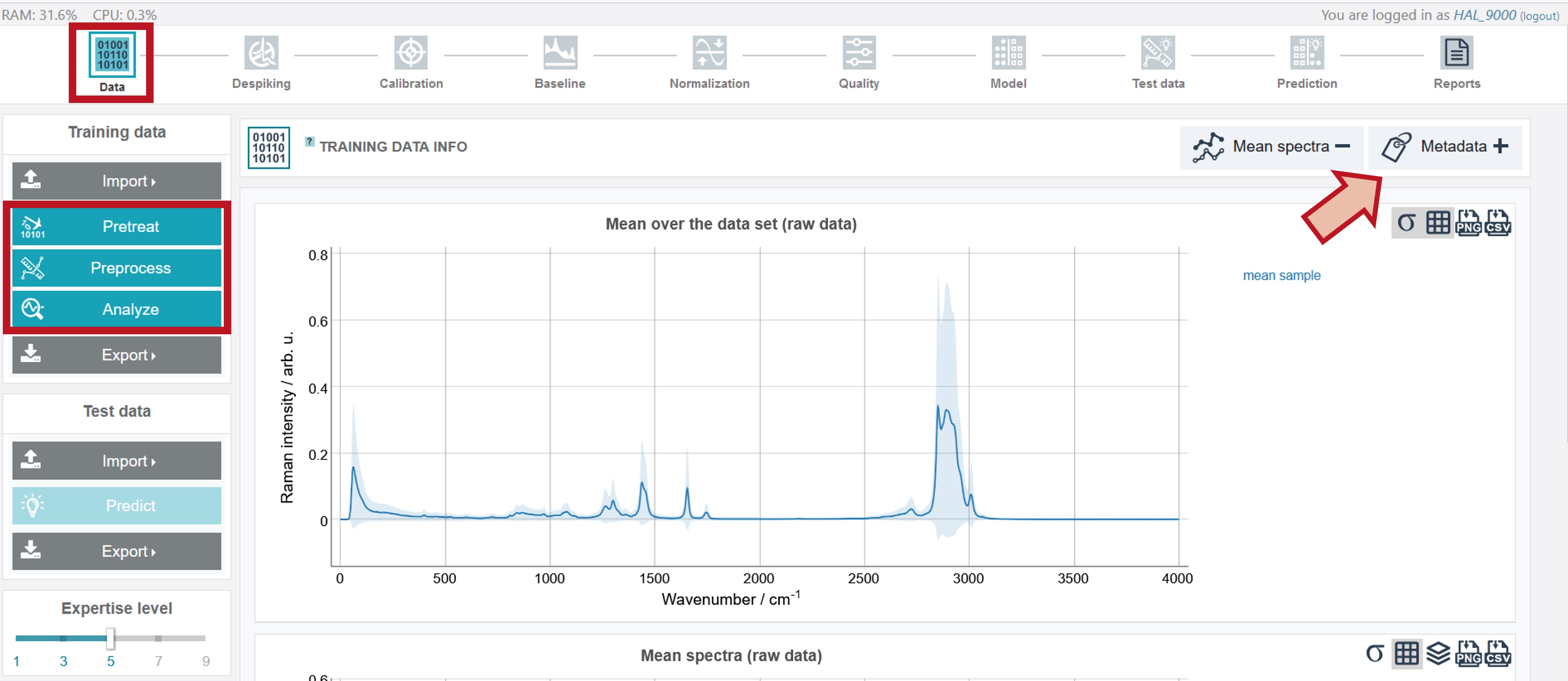
The appearance of the main interface depends on the chosen expertise level ( see Choosing your level of expertise). When starting the software for the first time or starting a new session, expertise Level 5 is set as default with the following main interface:
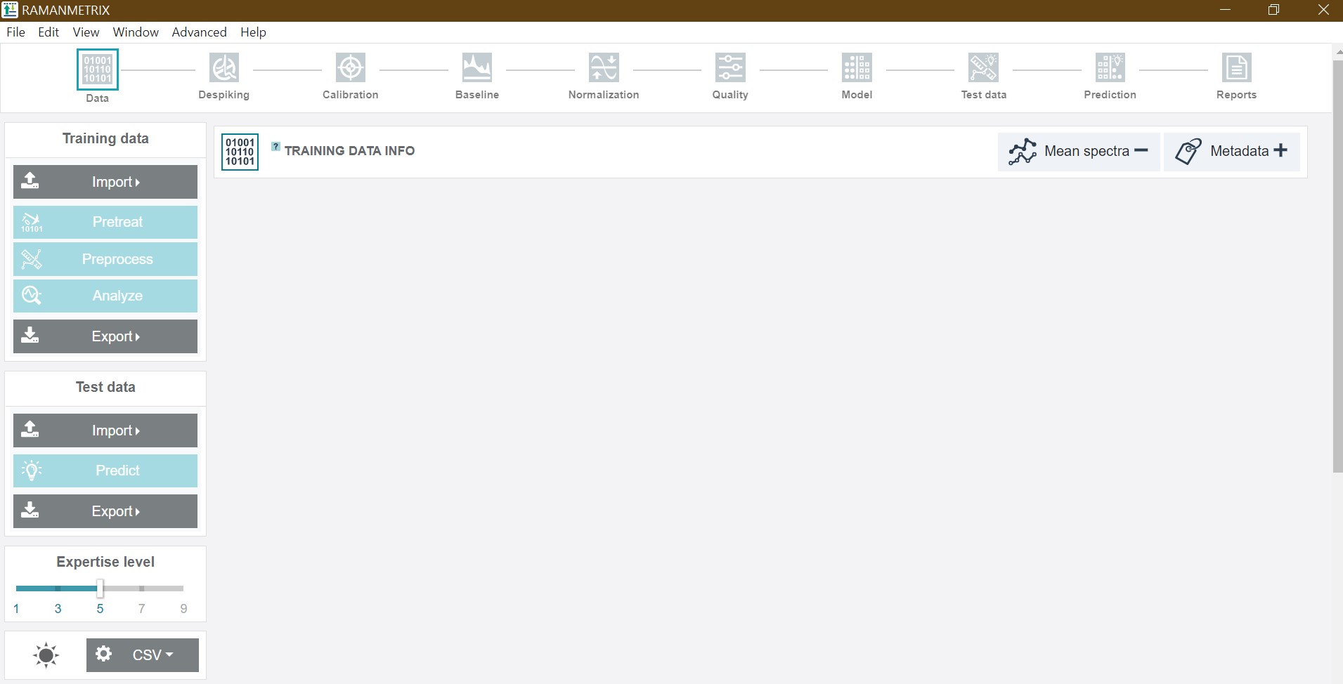
The left toolbar consists of the Import and Export buttons as well as the single-click-features for the * Training* and Test data. In addition, the slider for adjusting the expertise level, a dark/light -mode-button, and options for the *.csv file import can be found there.
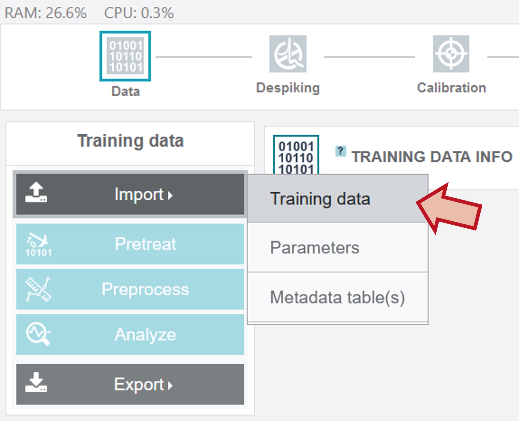
In the case of Training data, the respective dataset, a pre-saved parameter file and the metadata tables can be uploaded:
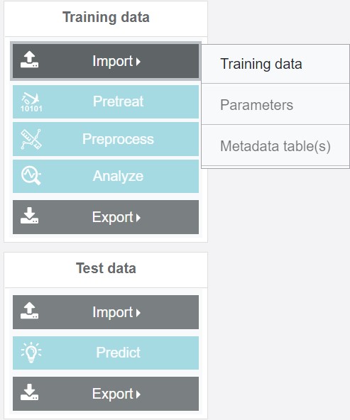
The parameter file contains all parameters, which were saved from a previous analysis (including preprocessing, pretreatment, quality filter and modeling). Please note: If the parameter file is saved after an intermediate processing step (e.g. just despiking and calibration were carried out) then either the default values or the set values from the last session are saved as parameters for the following steps and might need to be adjusted within the new analysis:
By clicking the Pretreat button on the left the pretreatment process, including despiking and calibration, is automatically conducted with the parameters from the previously uploaded parameter file.
By clicking Preprocess the whole preprocessing pipeline is automatically conducted (including despiking, calibration, baseline correction and normalization).
By clicking Analyze the whole preprocessing and modelling pipeline is automatically performed by just 1 click.
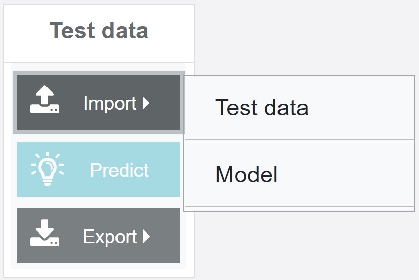
For the Test data, the respective dataset and a pre-built model can be uploaded and the model can be tested by just one click via the Predict button:
Via the upper function panel the individual steps of the data pretreatment, preprocessing and modelling pipeline can be accessed with the available functions also depending on the chosen expertise level. The individual functions will be discussed in more detail later on in this tutorial.

When setting the expertise level lower than 5 the main interface appears with a reduced set of buttons.
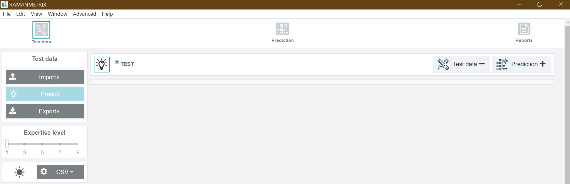

Level 1 is intended to carry out an easy and fast analysis of a test dataset based on a pre-built model with just 1 click. Thus, just the Test data toolbar on the left is available and no parameters can be adjusted. Also the upper functional panel is available in this case just in a reduced version.
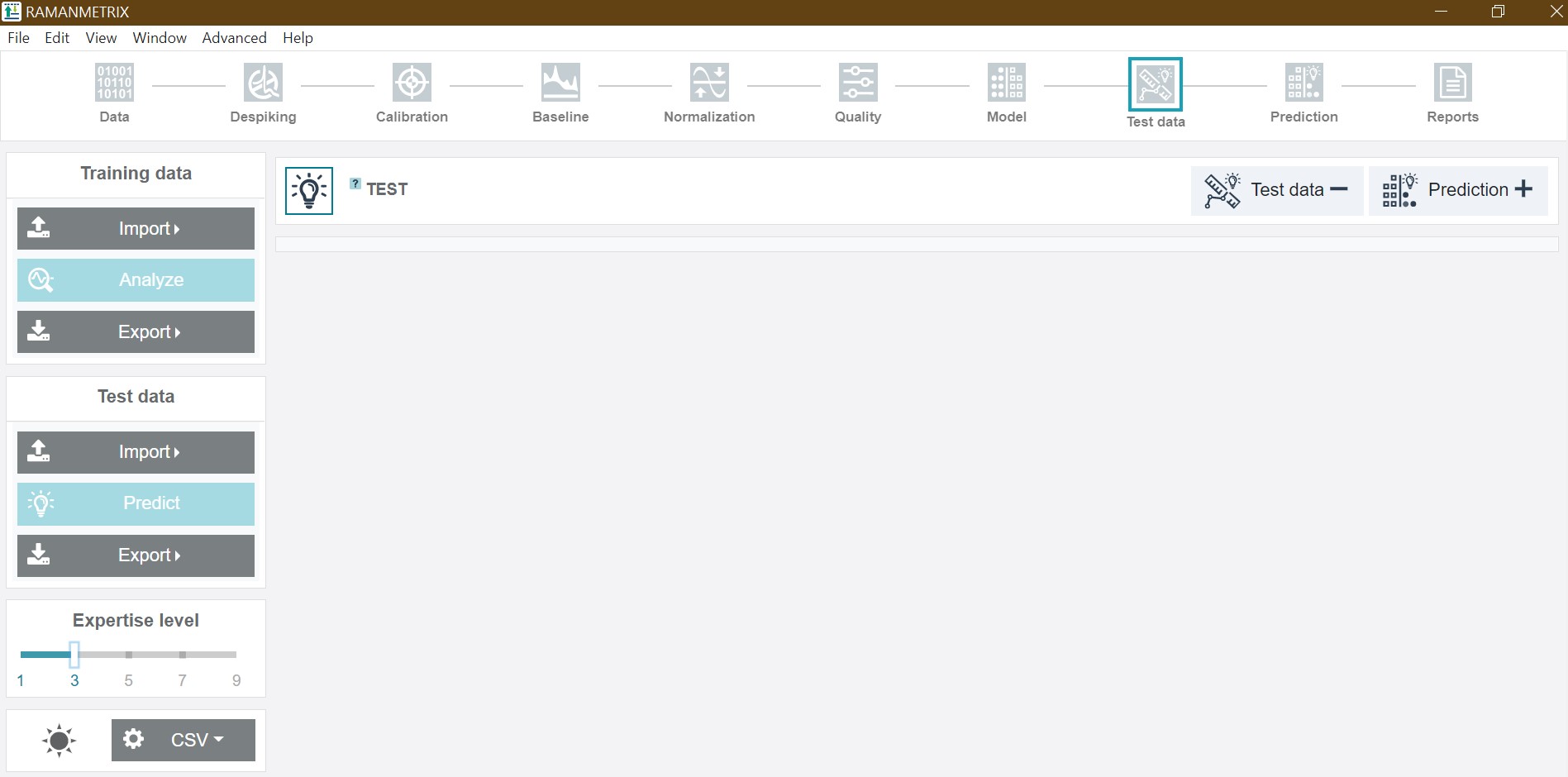
In addition to the test data analysis, Level 3 offers the possibility to build a model for a training dataset based on predefined parameters. Here just few options are adaptable.
For a more detailed description of the expertise levels see Choosing your level of expertise in the following paragraph.
Choosing your level of expertise
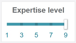
Depending on the tasks that you are working on and on your level of experience with preprocessing and analyzing Raman spectroscopic data, you should select one of the following expertise levels:
Level 1 is the most suitable for the test and identification tasks. This expertise level allows to import the * .pkl model file, import the test data (see Data Input) and perform the prediction in a single click without adjusting any parameters. For more details see Predicting test data.
Level 3, additionally to the functionality of the first level, makes it possible to preprocess training data and build a model on the training data with preset parameters. Either default parameters or parameters saved as a “.txt” file may be applied to the data. Only few options, such as presence of 2 spectra for each point (typical for BPE data) and a validation type (batch-out or 10-fold cross-validation) can be changed at this level of expertise.
Level 5 (default). Besides the options available on previous levels, this level provides controls for tuning spectral ranges at different steps of the preprocessing routine and a number of components used after the dimension reduction. Starting from this level of expertise, a step-by step execution of the data processing workflow is possible.
Level 7 makes possible to choose algorithms for baseline correction, normalization, and model construction. Advanced functionality becomes available to a user at this level, including a possibility to control data quality by setting various thresholds and averaging spectra according to a specified grouping.
Level 9 makes all the parameters, accessible. For example, advanced parameters for the calibration step, or a peak range for integrated intensity thresholding. At the model construction step, SVM cost and kernel become available.
PLEASE NOTE: While the selectable options are restricted at lower expertise levels, RAMANMETRIX retains full functionality at all levels.
Data import
RAMANMETRIX supports different data input formats including TXT and SPC files.
The spectral data can be imported via the Import button on the left function panel. To import the data the respective spectra should be provided together with a metadata table in a single ZIP folder where in the metadata table the measured spectra are specified in more detail. In addition to the ZIP data folders also previously saved parameter files or individual metadata tables can be imported.
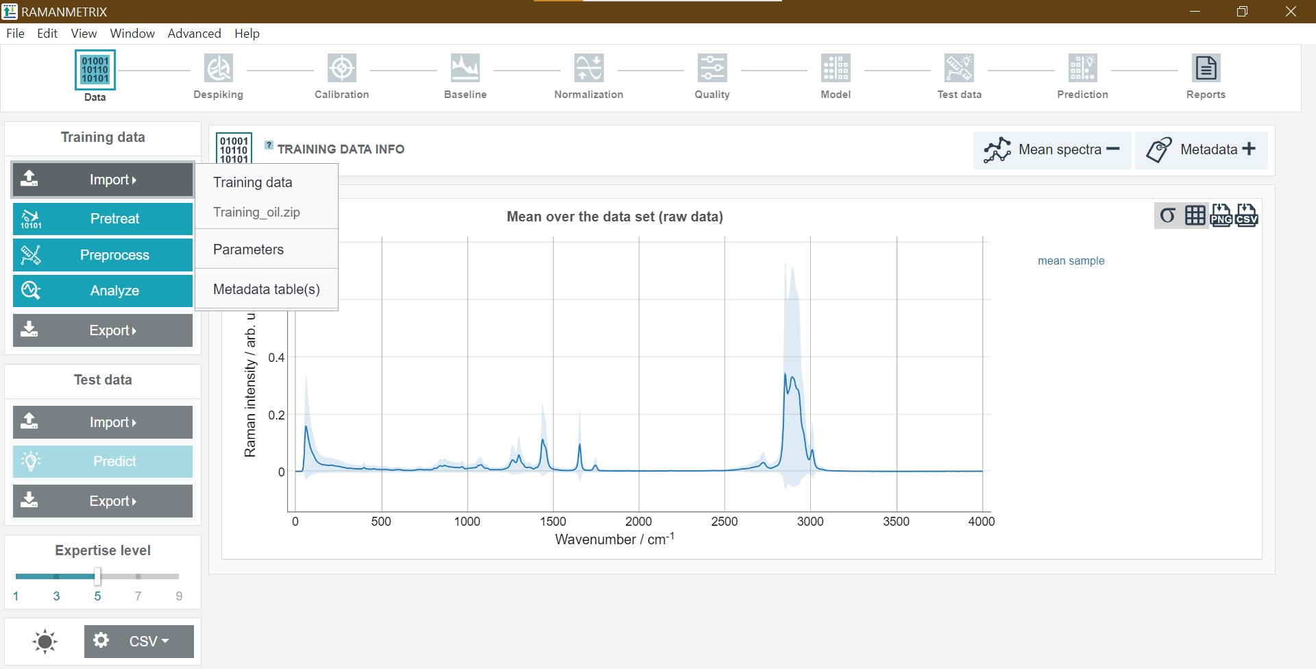
After importing the ZIP file a graph with the mean spectrum of all imported spectra and the mean class spectra is depicted in addition to the metadata info below.
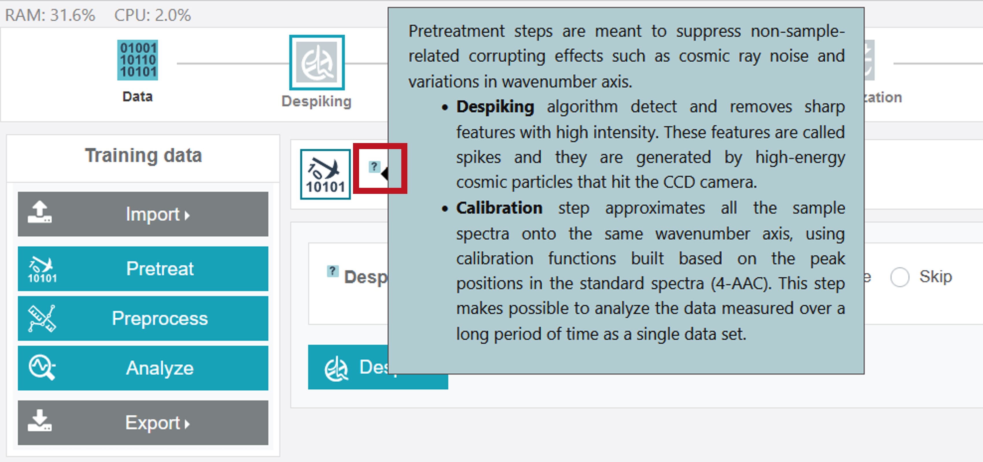
Infoboxes
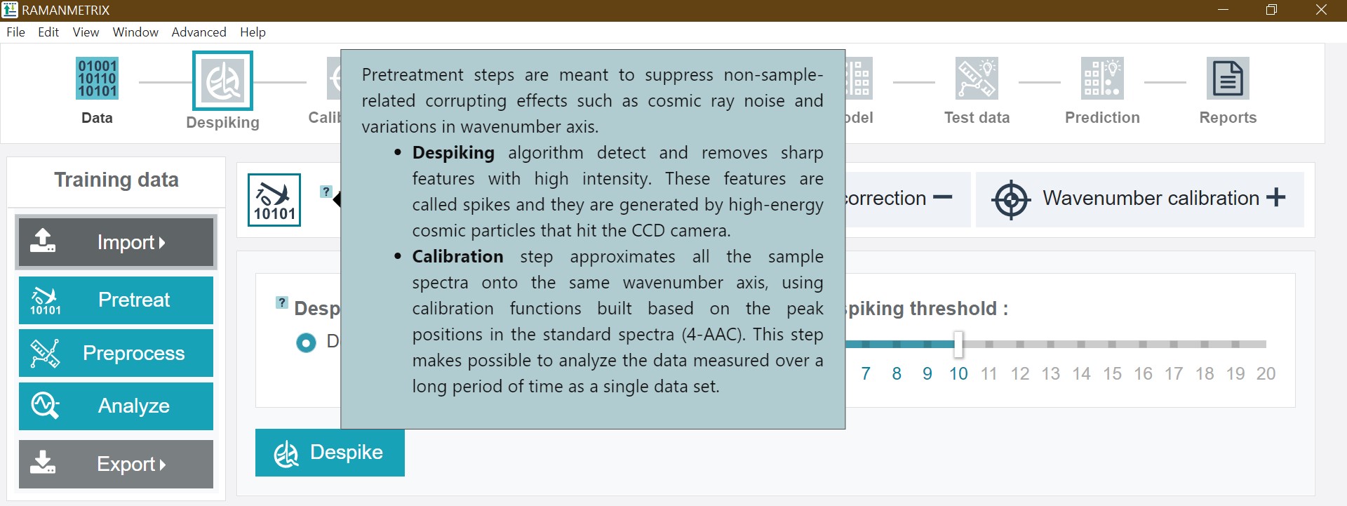
Infoboxes containing specific information and explanations of e.g. a respective processing step or method are marked by questionmark icons, which appear when moving the cursor over the icon.
Pretreatment step 1 - despiking
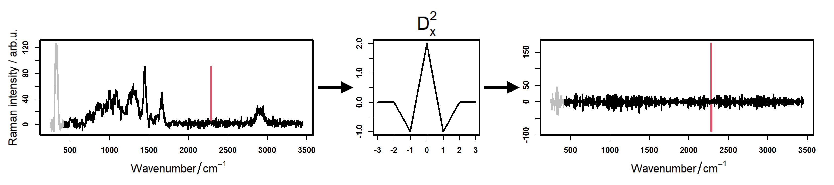
The despiking step serves to remove cosmic ray noise, which usually appears as sharp and intense signals.
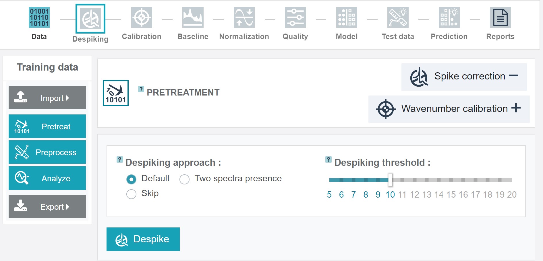
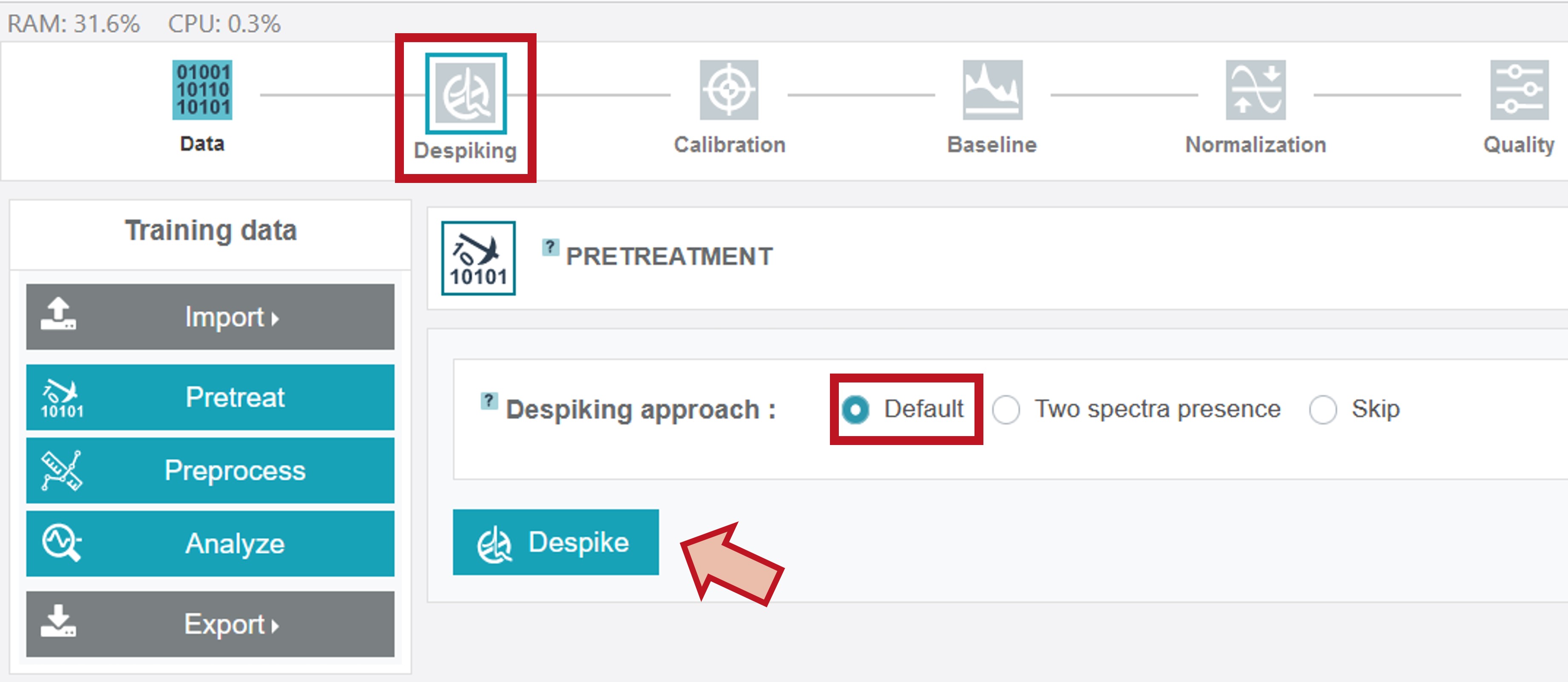
RAMANMETRIX offers different options for despiking:
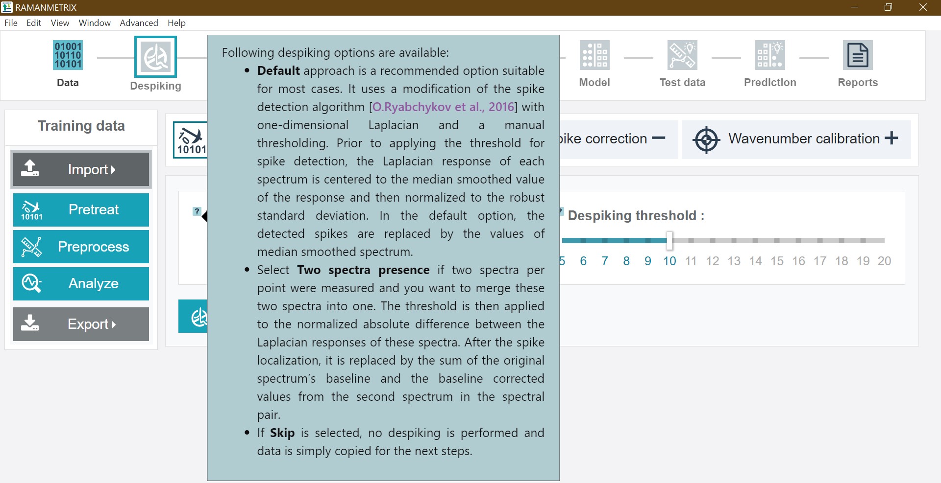
- When choosing Default an algorithm based on an one-dimensional Laplacian combined with a manual thresholding is applied. Detected spikes are replaced by the values of the median smoothed spectrum. This algorithm is the recommended option and suitable for most cases.
Two spectra presence can be applied when two spectra from one point were measured. In this case an averaged corrected spectrum is calculated.
If the despiking was already applied before this step can be also skipped (Skip).
Pretreatment step 2 - calibration
RAMANMETRIX provides an additional possibility for the spectral calibration including wavenumber, dark background, and intensity correction steps. The wavenumber calibration is particularly important if spectra for the analysis were measured on different spectrometers in order to approximate the spectra to the same wavenumber axis.
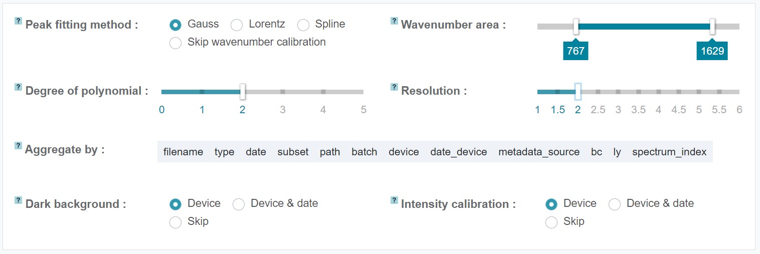
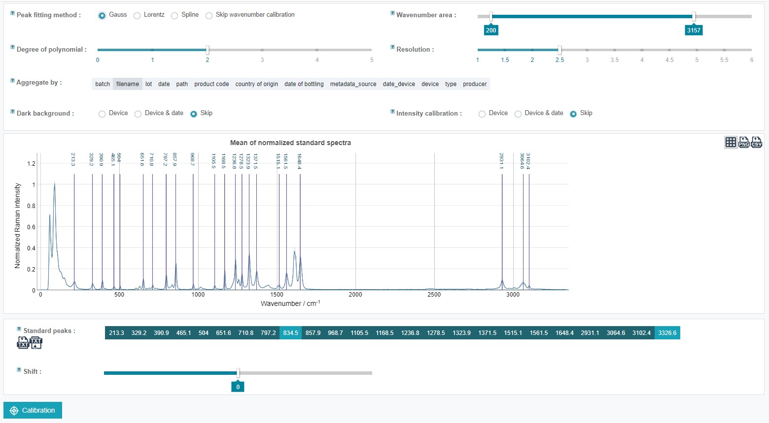
The RAMANMETRIX wavenumber calibration procedure is based on the acquired spectrum from a reference substance, which needs to be measured for each used Raman spectrometer and has to be referred in the metadata table. In addition, it's recommended to measure the reference substance also on each new measurement day and after changing spectrometer settings, e.g. when using another grating or changing the spectral region. The peak positions of the measured reference substance are fitted and compared to the standard peak positions of this substance. For the fitting RAMANMETRIX offers three different options for peak shapes - Gauss, Lorentz, and Spline - and a manual adjustment of the degree of polynomial.
The standard peak values included in RAMANMETRIX are those for (4-acetamidophenol) (paracetamol). However, it's also possible to use other substances as reference. For this, the standard peak values of the respective substance can be uploaded as txt file at Standard peaks. In this case, the paracetamol txt file can be used as template, which can be also downloaded under Standard peaks. Not all standard peaks need to be included for the calibration, but can be selected manually by choosing the respective numerical values. It is recommended to include just the peaks that are clearly visible. If the peak positions are too far from the tabled positions, the wavenumber axis can be manually shifted with the slider at Shift.
Also a dark current background (the signal obtained with closed shutter) subtraction is possible within RAMANMETRIX. It is not required if no intensity calibration is applied and the baseline correction is carried out in the next step of the RAMANMETRIX preprocessing pipeline. To subtract a measured dark background, the respective reference spectrum must be included in the data zip folder and a column with “dark_bg” must be added in the metadata table where the respective file must be marked with "True" and the rest of the data with "False".
To carry out an intensity calibration an intensity reference must be provided. The respective intensity standard spectrum must be included in the data zip folder and a column with “standard_intensity” must be added in the metadata table where the respective file must be marked with "True" and the rest of the data with "False". In addition, the intensity calibration reference standard values have to be provided with their respective wavenumber positions or as a set of polynomials in txt file assigned as “calib_response”, which can be uploaded together with the standard peak txt file.
The wavenumber calibration can be also skipped. In this case the standard spectra are ignored, but the spectra are approximated to a new linear wavenumber axis. If no dark background or intensity standard spectra are assigned in the metadata table these steps are automatically skipped.
An additional option in RAMANMETRIX is to select the wavenumber range within which the calibration should be applied. This can be done by the respective sliders at Wavenumber area.
Preprocessing step 1 - baseline correction
The preprocessing steps are intended to standardize the data by minimizing/suppressing variations in the fluorescence background and the signal intensity.
The baseline correction is an important step in order to increase the quality of the data analysis model. During the baseline correction the fluorescent background is estimated by an algorithm. For this RAMANMETRIX offers two options - a SNIP (sensitive nonlinear iterative peak) and EMSC (extended multiplicative signal correction) algorithm. The SNIP algorithm is a robust iterative method to estimate the background. Here, at the first iteration smoothing is applied in order to reduce the influence of noise in the spectra. The number of iterations is manually adjustable. It's recommended to set a higher number of iterations for spectra with wide peaks and high resolution. The principle of the EMSC (extended multiplicative signal correction) algorithm is that the spectra are equalized to a reference spectrum. If no reference spectrum was recorded and is addes as “reference_sample” column of the metadata table then the mean spectrum over the training dataset is used instead of the reference.
Preprocessing step 2 - normalization
The normalization is intended to minimize variations in the spectra caused e.g. by inaccurate focus. This step can usually be skipped when applying the EMSC algorithm in the previous step. RAMANMETRIX offers five different normalization types. In addition, it's possible to include and exclude specific areas to the normalization by sliders.
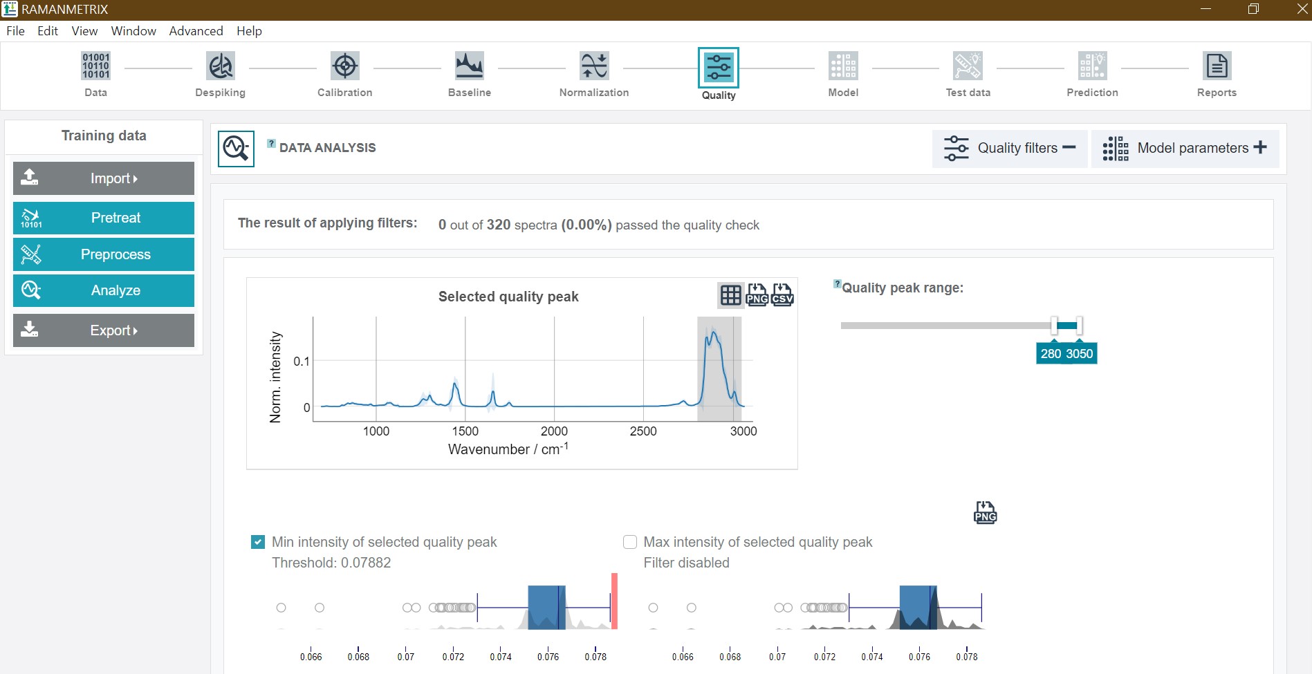
Quality filters
For the Expertise Levels 7 and 9 additional quality filters are available. They enable sorting out low-quality and corrupted spectra and thus increase the model outcome. The filters can be activated by clicking on the checkboxes or boxplots. The threshold of the filters is adjustable by the red bars, which appear after the activation of a respective filter option. It is also possible to apply several filters in parallel. RAMANMETRIX offers eight different quality filter options:
- Filtering the data based on the minimum and maximum integrated normalized intensity values defined by a set quality peak with adjustable peak range. After changing the wavenumber range, Update quality peak must be clicked.
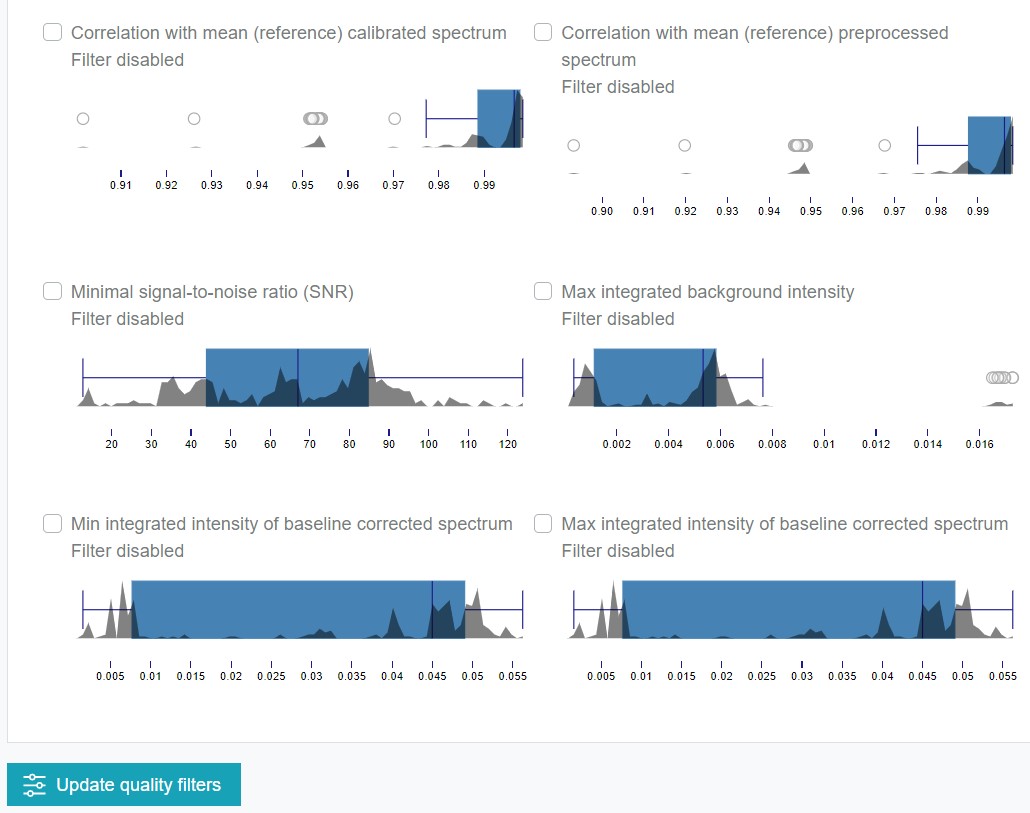
Correlation with a reference spectrum (defined as “reference_sample” column in the metadata table, otherwise the mean over the training dataset is applied). It is possible to choose if this reference spectrum should be referred after the pretreatment (calibration) or the preprocessing (normalization). Applying this filter option is especially recommended, if a large number of outliers is expected.
Minimum value of the signal-to-noise ratio (ratio between maximal intensity and a standard deviation of noise). This filter is based on estimating the signal as the mean of the smoothed spectrum while the noise is estimated as difference between the original and the smoothed spectrum.
Maximum of the integrated intensity from the estimated background. If the EMSC algorithm was applied for the background correction within the preprocessing, an intercept model coefficient is used as the integrated background intensity. In case of skipping the background correction before, the minimum value within the spectrum is applied.
Minimum and maximum value of the integrated intensity of the baseline corrected spectrum.
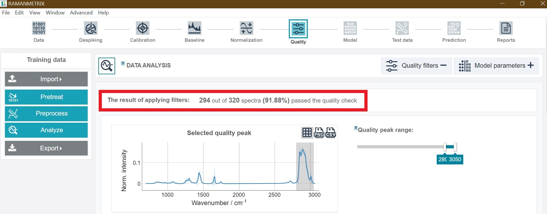
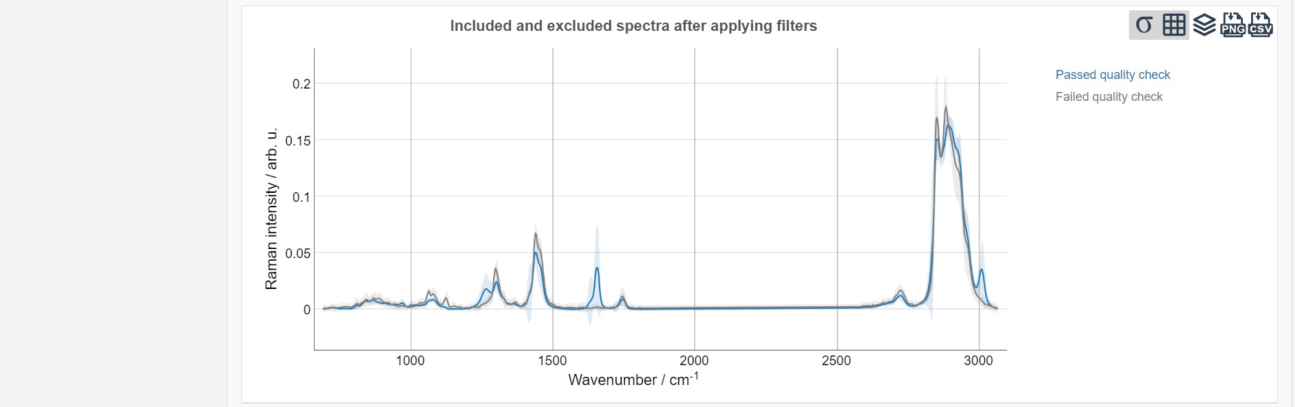
The results of the quality check are presented as numerical value in the top showing how many spectra passed the quality check. In addition, a plot of the mean spectra from the data which passed and failed the quality check is available.
Modeling
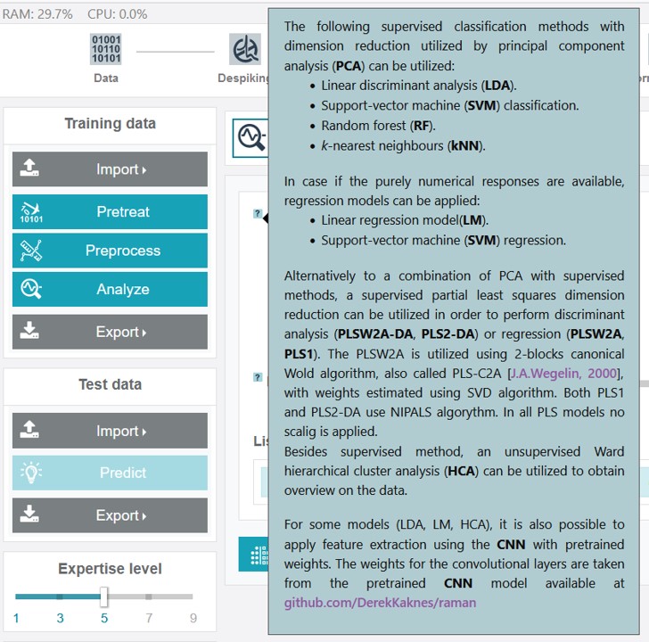
RAMANMETRIX offers various model options for a supervised classification and regression analysis as well as two model options for an unsupervised cluster analysis.
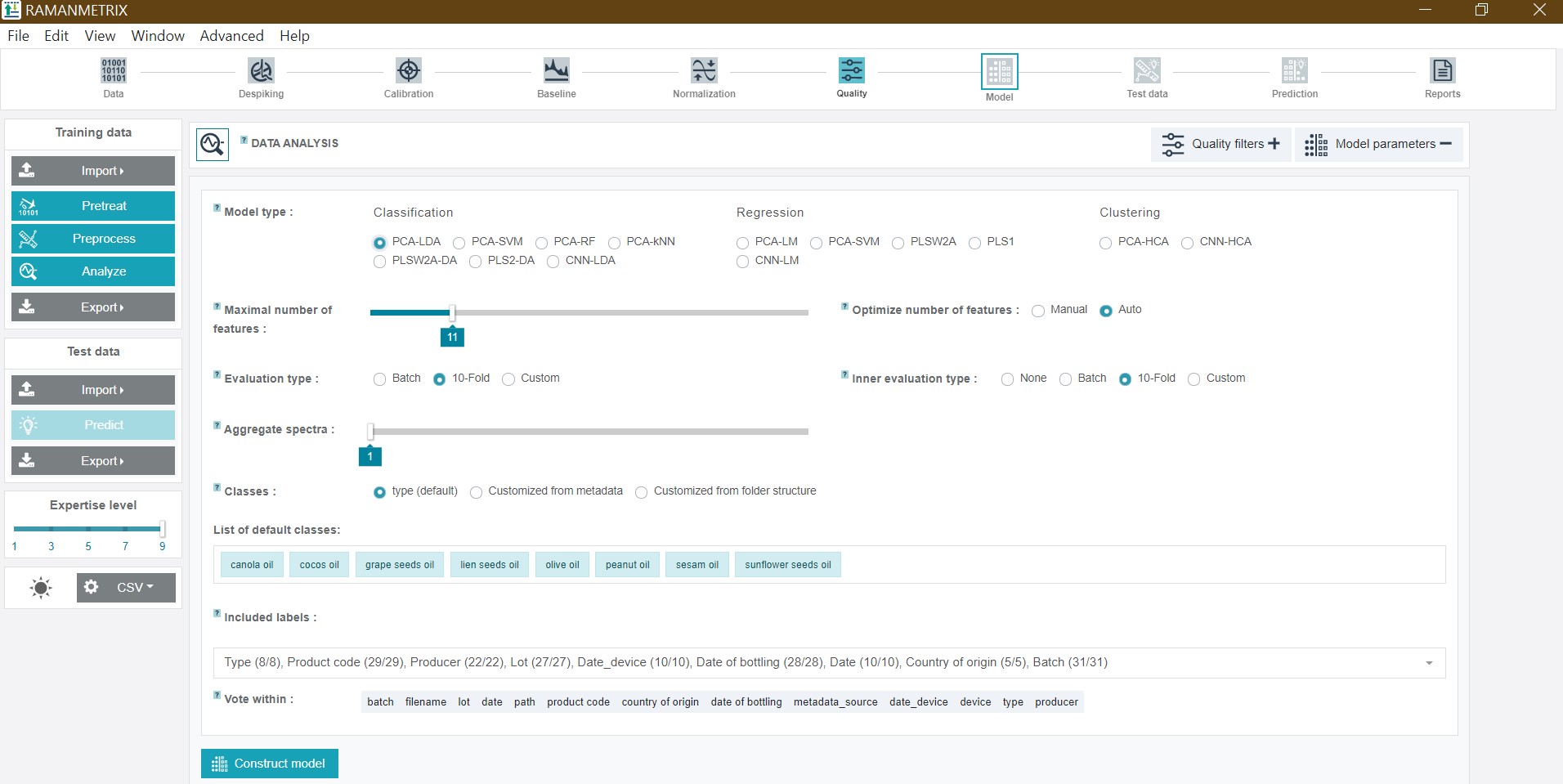
The available model types for the classification analysis are:
- LDA (linear discriminant analysis)
- SVM (support vector machine)
- RF (random forest)
- kNN (k-nearest neighbors)
- PLSW2A‑DA and PLS2-DA (partial least squares discriminant analysis with two different implementations)
The available model types for the regression analysis are:
- LM (linear regression model)
- SVM
- PLSW2A and PLS1 (partial least squares regression with two different options)
For the unsupervised clustering analysis a HCA (Ward hierarchical cluster analysis) is implemented in RAMAN METRIX with an adaptable number of clusters.
Except for the PLS-based models (as the PLS algorithm is based on a supervised dimensionality reduction), all methods contain a preceding dimensionality reduction to avoid overfitting. For this two options are integrated - the PCA ( principal component analysis) and the CNN (convolutional neural network) approach.
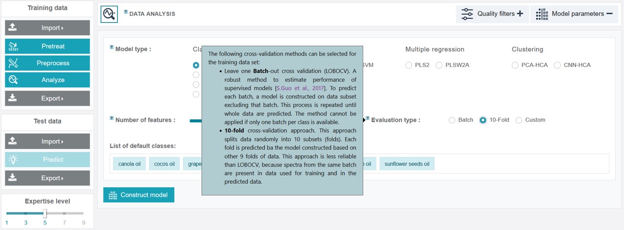
To validate the supervised models RAMANMETRIX offers a 10-fold or a leave-batch-out cross-validation approach. Additionally, the evaluation can be customized by selecting class and batch labels based on the metadata table, whereas also multiple labels can be chosen in parallel. Via “Included labels” it is possible to exclude spectra corresponding to any value of any of the metadata columns. Only the spectra which satisfy all the conditions will then be considered for the model construction.
In case of the regression it is possible to select any of the numeric columns from the metadata as a response.
Analyzing training data
The data analysis functionality is available for Expertise levels above 1 ( see Choosing your level of expertise). If a lower experience level is set, only the testing is possible (see Predicting test data).
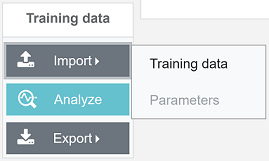
To import the training data, find a panel named “Training data”, click Import --> Training data and select a pre-structured ZIP file (see Data Input).
To analyze data in a single click, use the Analyze button (left panel). After clicking the button the analysis process will begin step by step and the results for each data processing step can be accessed by clicking on the icons at the upper toolbar of the program window:

The summary of the analysis can also be accessed in a form of a complete report by clicking at the Report icon at the stepper panel. Other results can be exported through the “Export” menu at the left panel.
Specific pre-set parameters can be imported as a text file through "Import -> Parameters". Furthermore, parameters can be manually adjusted for each data processing step. A set of the adjustable parameters depends on the selected expertise level (see Choosing your level of expertise).
Predicting test data
To import the test data, find a panel named “Test data”, click Import Test data and select a pre-structured ZIP file ( see Data Input).
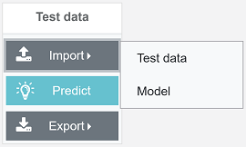
The test data predictions can be generated using either a model constructed from training data or using a pre-stored model. How to construct the model is described in Analyzing training data. To import a pre-built model, find a panel named “Test data”, click Import Model and select *.rspa file. The pretreatment and the preprocessing of the test data are performed with the same parameters that were used for the training data. When a pre-stored model is used, these parameters are embedded in the model and cannot be changed by the user.
After importing or generating the model and importing the test data, simply click “Predict” at the “Test data” panel. To see more details, please click at the icons Test data and Prediction at the upper stepper panel.

The summary for preprocessed data can be found in a form of a report. Other results can be exported through the “Export” menu at “Test data” panel.
Interactive plots
To change the styles of the graphs before saving and highlight the information of interest, the following tools can be used:
Zoom: click on the canvas and hold to expand the area that should be zoomed in. Work in both vertical and horizontal directions. Double click – reset to initial scale.
Lock one spectrum: click on one spectrum to highlight it (R.terrigena DSM 2687) and click on the empty space on the canvas to unlock it.
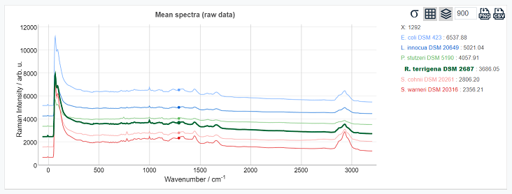
Remove/Add spectra: hover on the legend area and use the checkboxes to hide/add spectra
Legend: hover on the spectrum label to highlight it on the canvas. Come back to the canvas to examine the value in a hovered point.
Top toolbar functionality:
| Icon | Action |
|---|---|
 | Save high quality image in a PNG format. |
 | Save data in a CSV format to plot it by yourself in a different program |
 | Add offset on Y-axis to better distinguish nearby spectra |
 | Make invisible a colored area on the canvas which shows selected wavenumbers range |
 | Add/remove standard deviation |
 | Add/remove grid on the background |
Examples
Classification task edible oils (Expertise Level 5 / Online Version)
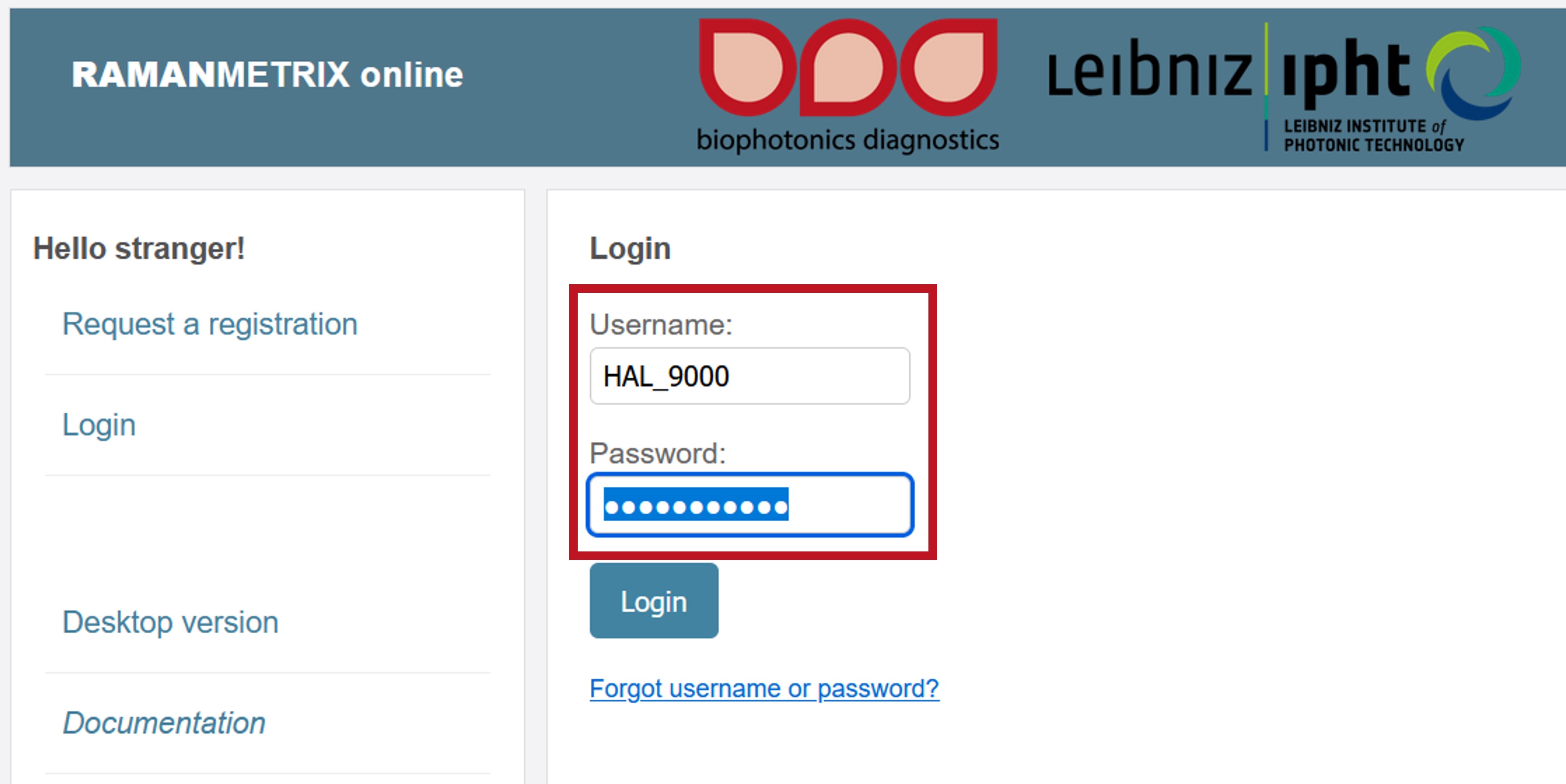
Login
Users with license can log in here with their username and password:
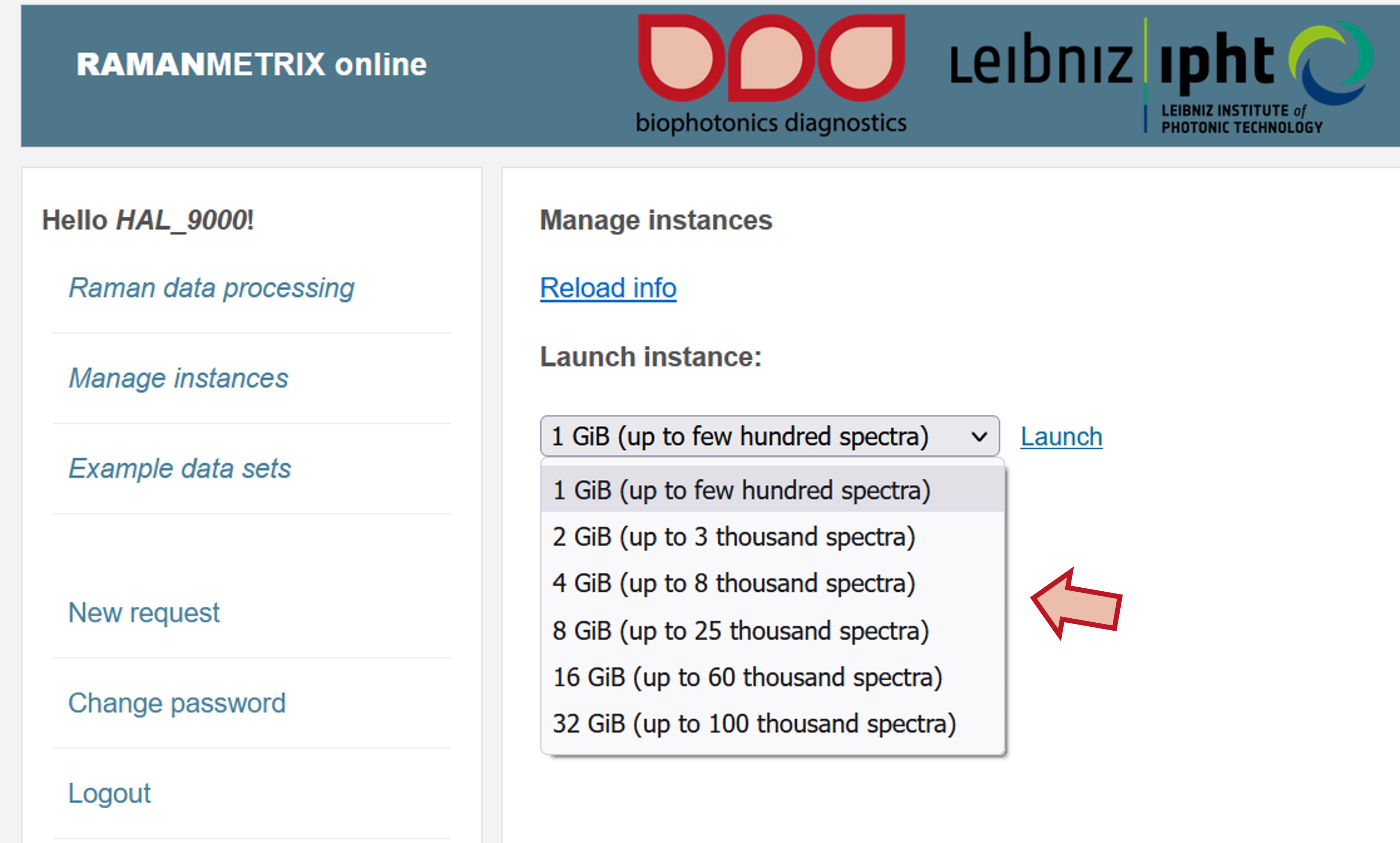
Instance
Choose an instance size that fits the size of your data set and click Launch.
User interface
The RAMANMETRIX user interface appears after a short initialization at Expertise Level 5 set as default. This level already offers all essential tools for an appropriate data analysis and model construction.
Import training data
To import the training data set “Training_Oil” click the Import button on the left bar, then click Training data and choose the respective zip-file on your computer.
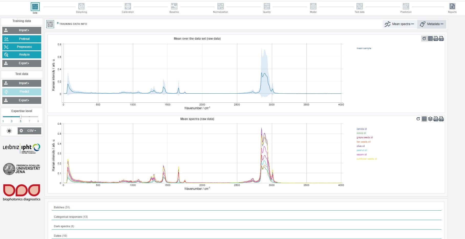
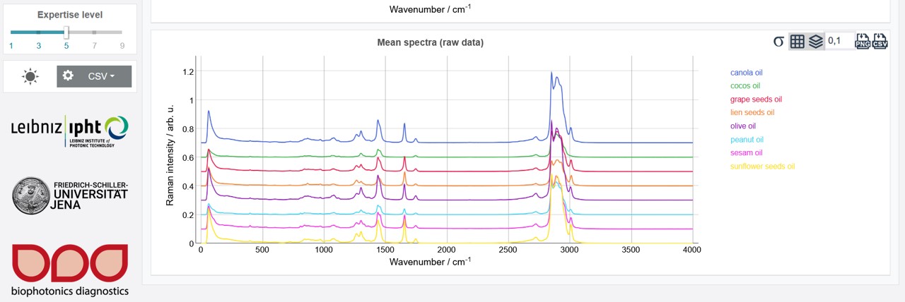
After a successful upload the button Data in the upper toolbar appears green and the mean spectrum over the whole data set as well as the mean spectra of all individual oil types are shown. Additionally, the metadata information can be accessed by clicking the "+" on Metadata on the right side under the upper toolbar. To receive an optimum model, a preprocessing and pretreatment of the raw data is recommended. If pretreatment and preprocessing parameters are already available from a previous analysis, these steps can be carried out fast and easy via the Pretreat and Preprocess buttons on the left. When clicking Analyze the whole modelling process is automatically carried out. If no respective parameters are uploaded the values of the last session are applied or (if the first time using the software) the default values. These pretreatment, preprocessing and modelling parameters can be adjusted for new datasets step by step via the upper toolbar. How to proceed with this for the oil training data set is shown in the following.
Pretreatment - Despiking
The pretreatment process includes a despiking and calibration approach. Further detailed information for specific treatment/modelling steps and options are marked with a ? in the software. By sliding with the cursor over a ? symbol a box with the respective infos and descriptions opens.
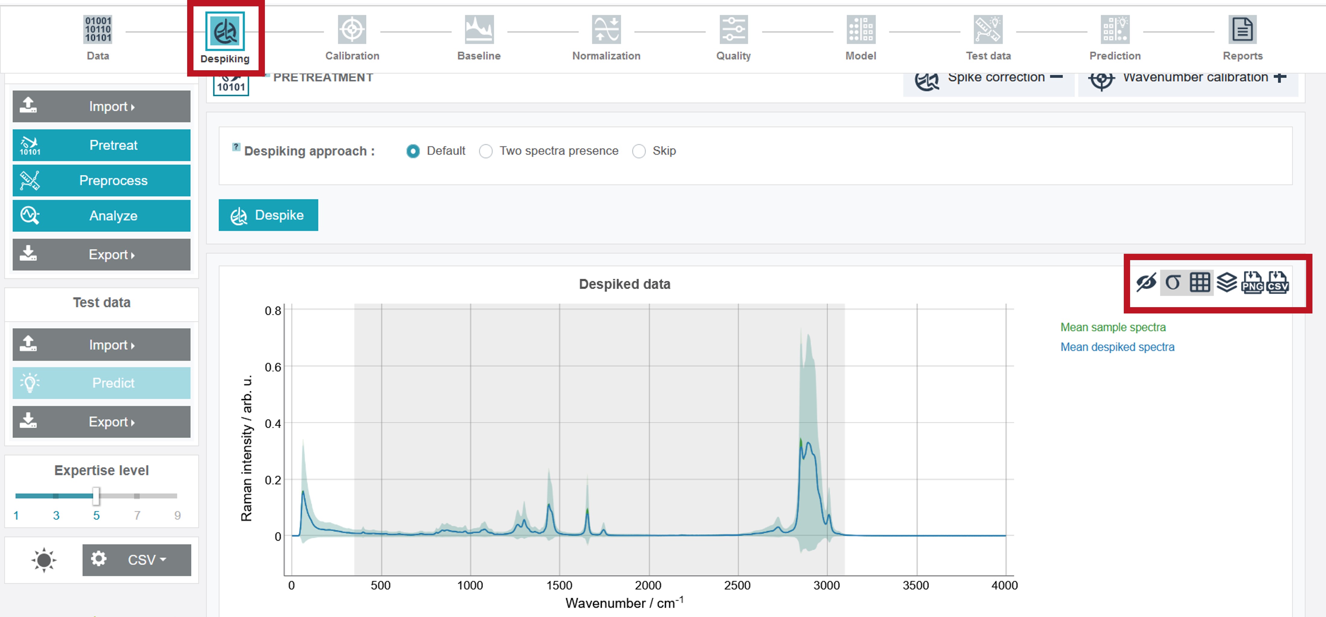
The currently selected processing option in the upper toolbar is marked by a green frame with a light grey/white colored symbol if the chosen step was not carried out yet. Different despiking approaches are available. For the oil training dataset chose Default and then click Despike.
The completion of the process is marked by a green filled and black colored symbol of the currently selected processing option. In addition, the graph with the despiked mean spectra (compared to the raw data) is depicted. The graph can be customized by the toolbar right of the spectrum, where e.g. standard variation can be shown or the spectra can be plotted offset. Furthermore, the spectra can be either exported in png or csv-format.
Pretreatment - Calibration
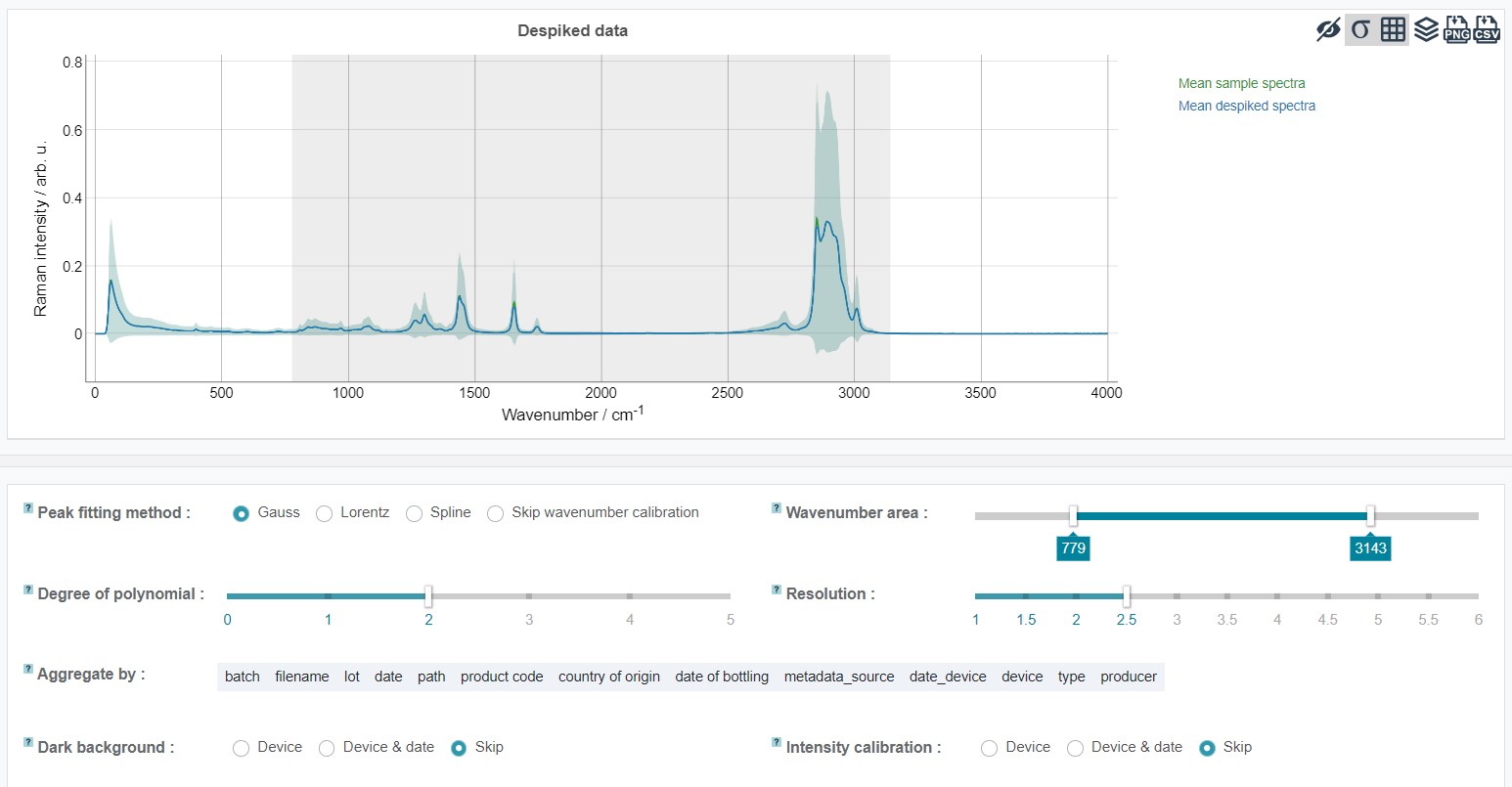
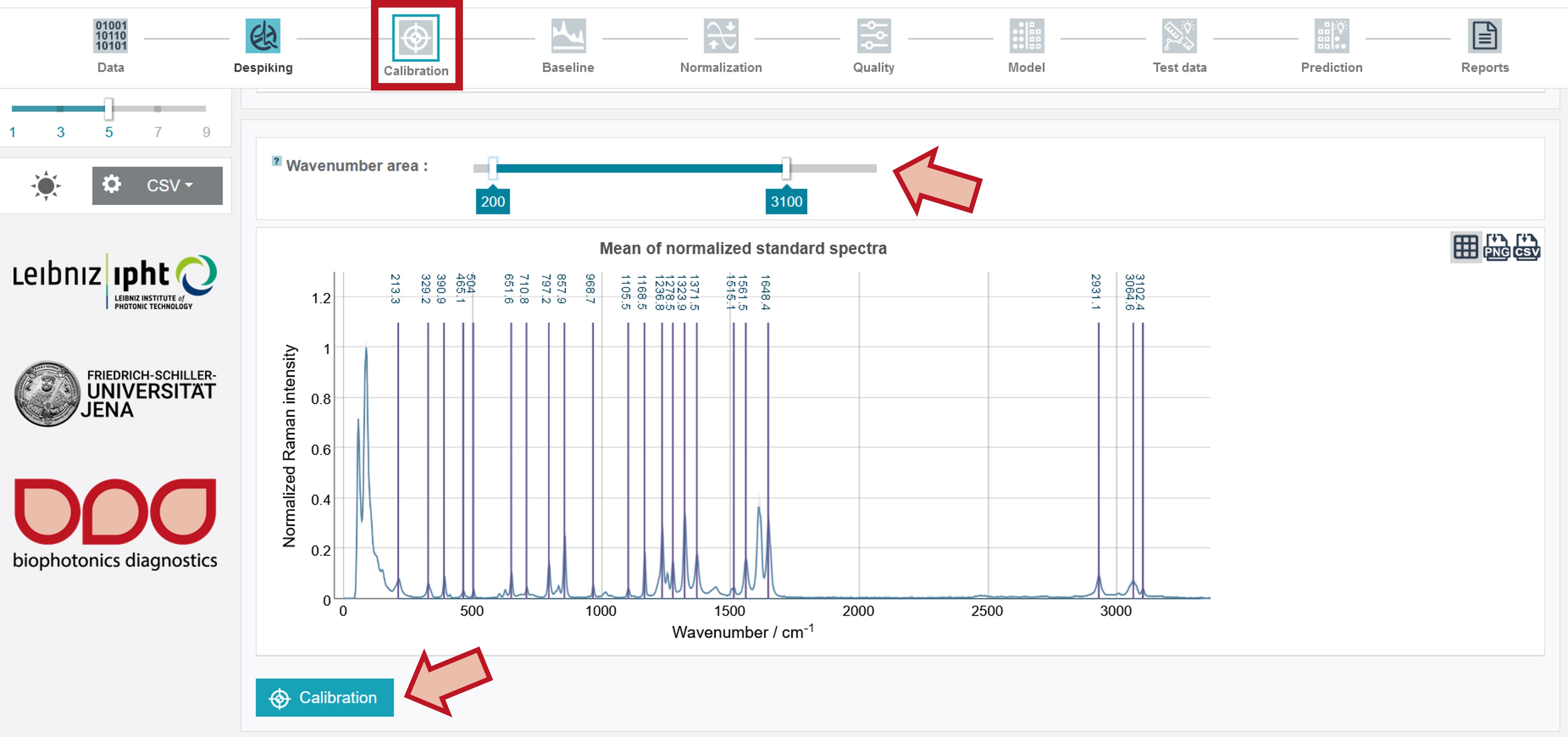
For the calibration 4-acetamidophenol (paracetamol) is applied as calibration standard. The respective peaks used for the calibration are marked with their wavenumber in the Raman spectrum. For calibrating the oil training dataset set the wavenumber area from 200 to 3,100. This can be done by sliding the cursors and an additional fine-tuning by the arrow keys on the keyboard. Then click Calibrate.
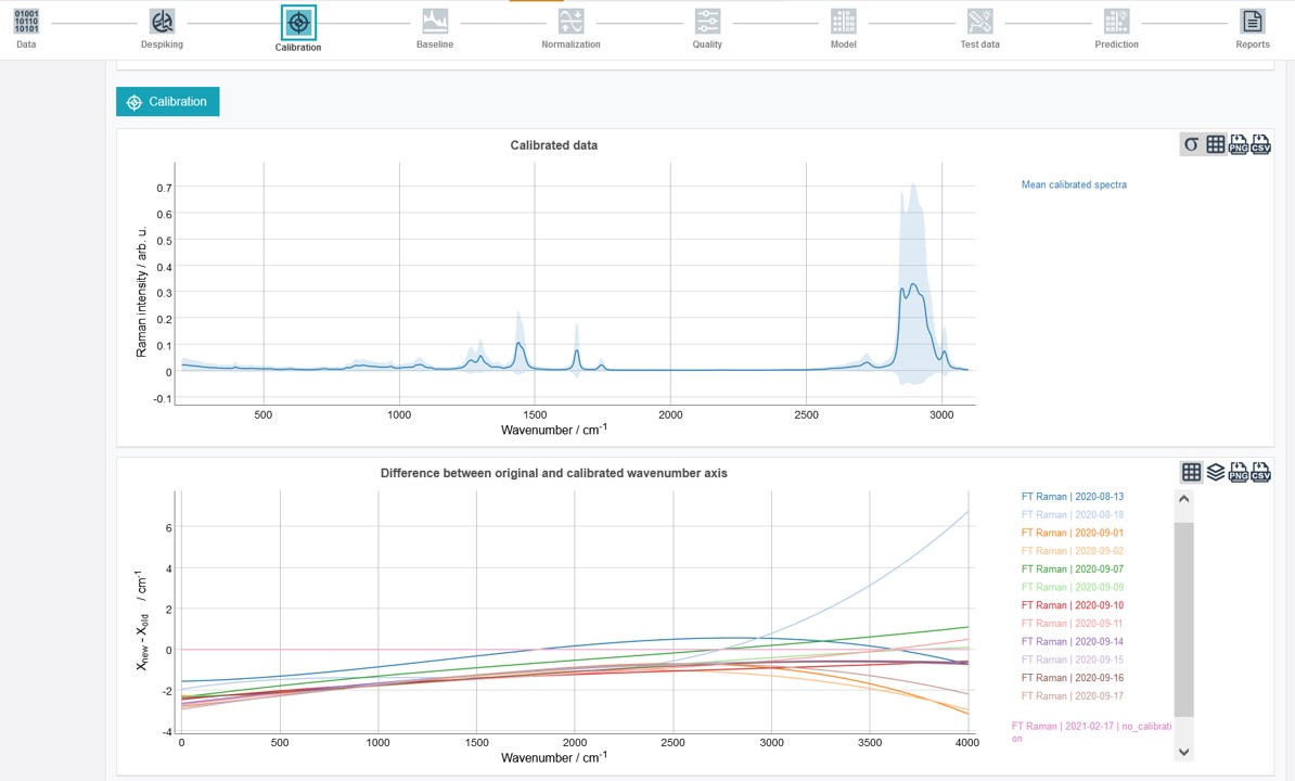
The calibrated mean spectrum and a graph depicting the difference between original and calibrated wavenumber axis appear after completing the calibration.
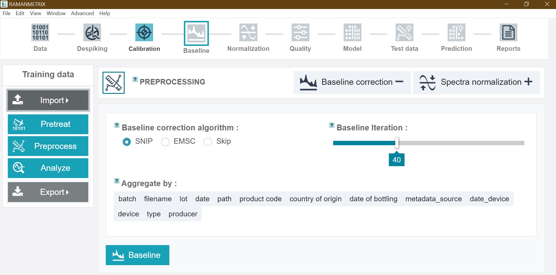
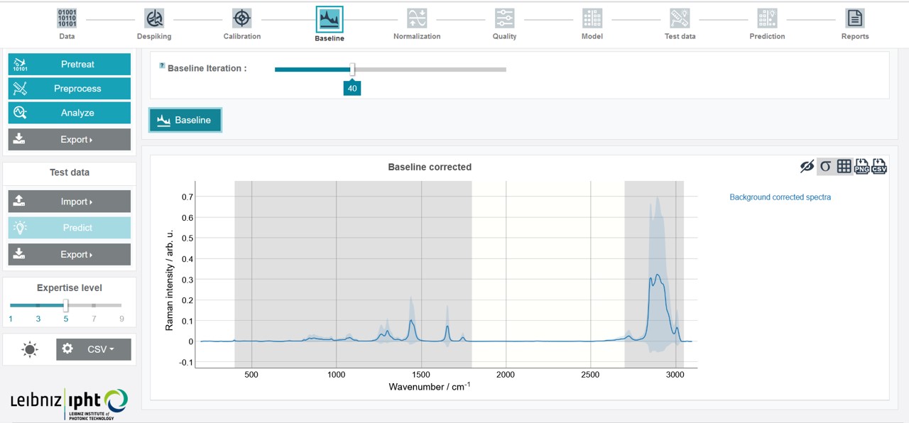
Preprocessing - Baseline correction
The preprocessing includes a baseline correction and normalization of the spectra. The number of baseline iterations can be adapted by sliding the cursor. For the oil training dataset choose 40 iterations and click Baseline.
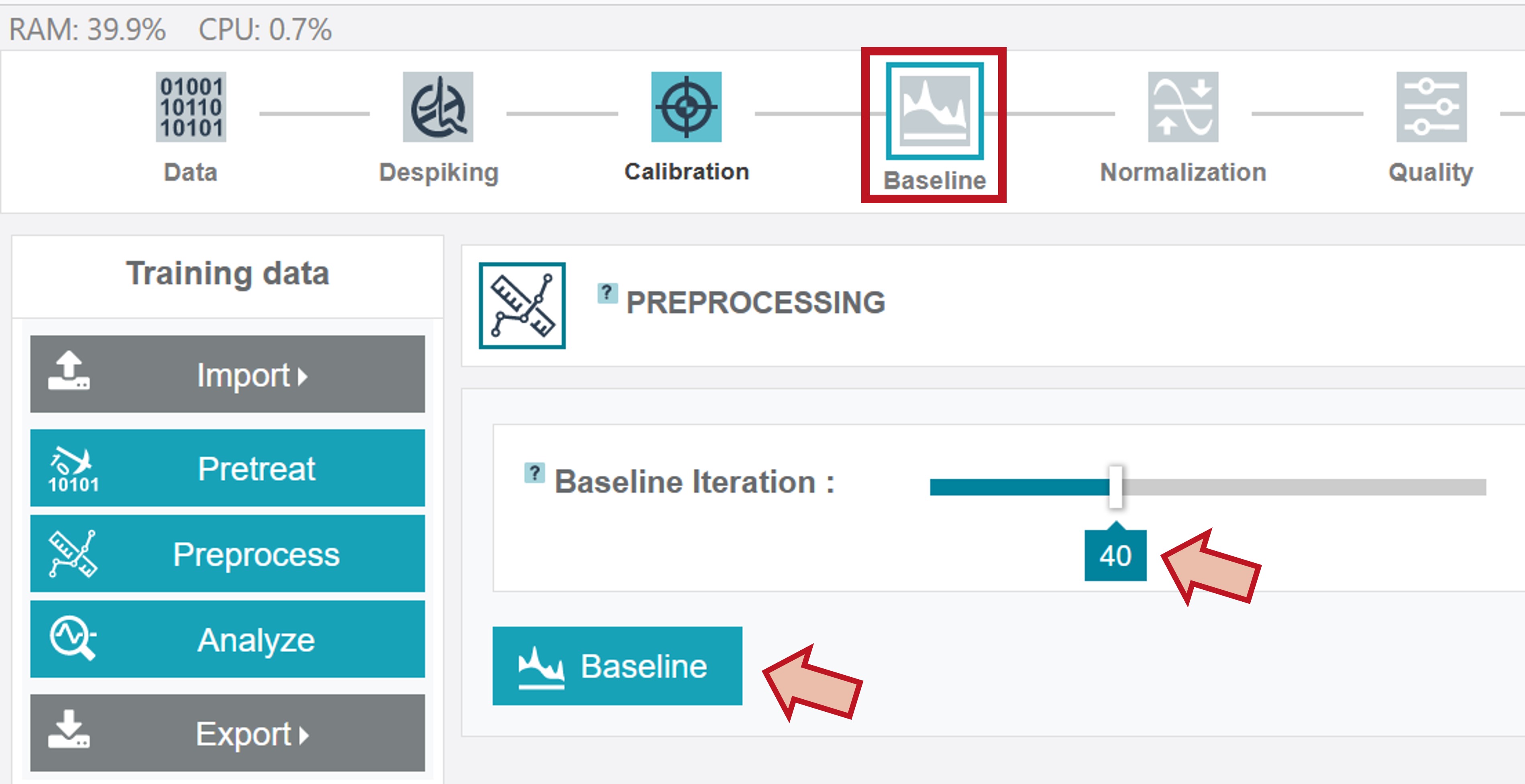
After finishing this step the baseline corrected mean spectrum is depicted.
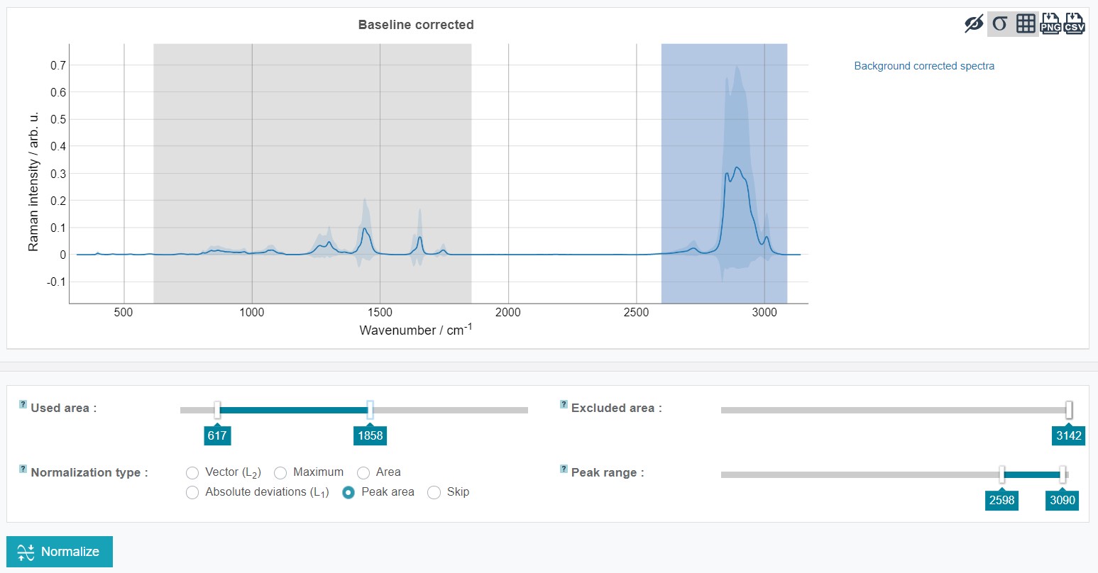
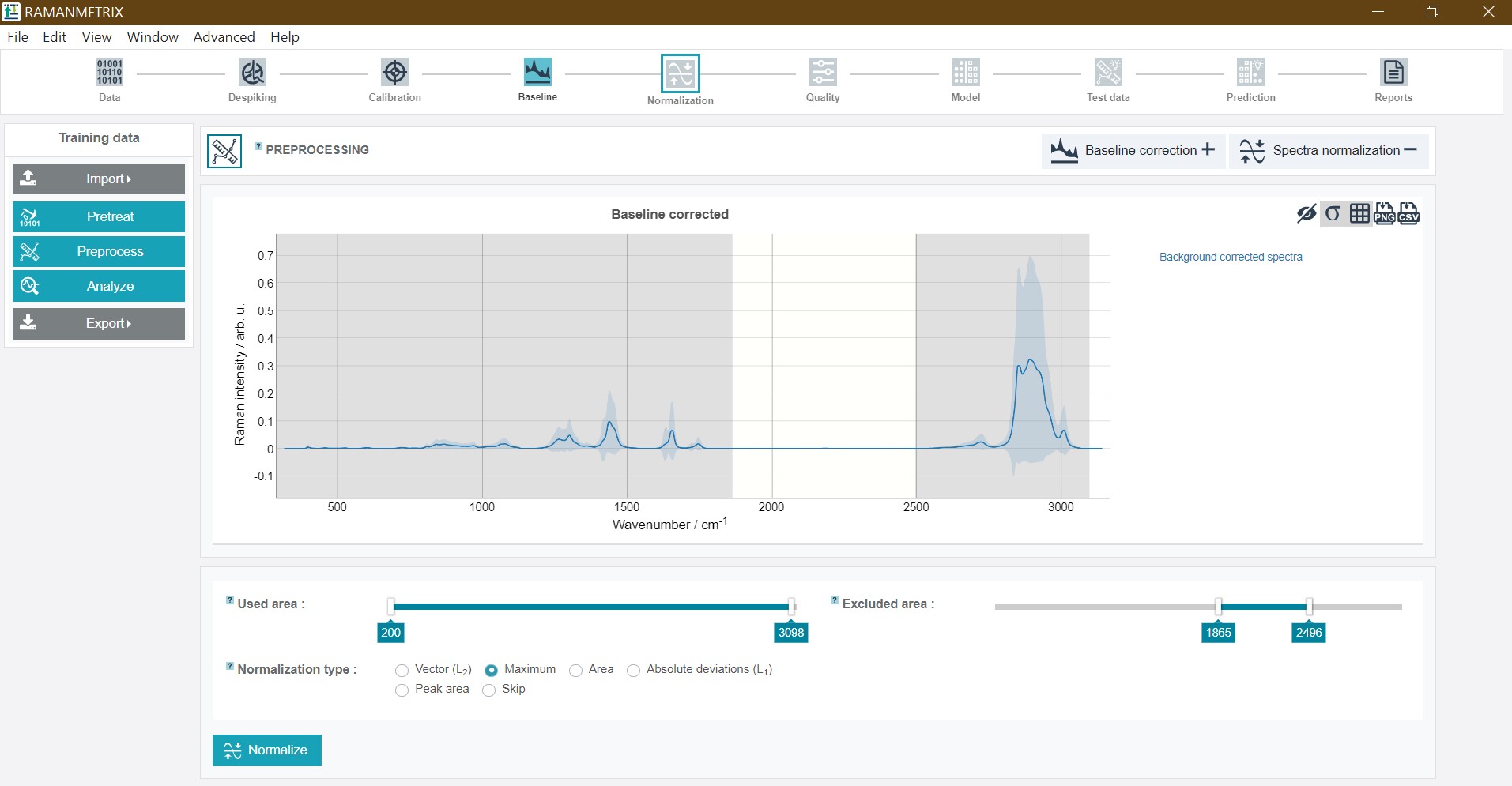
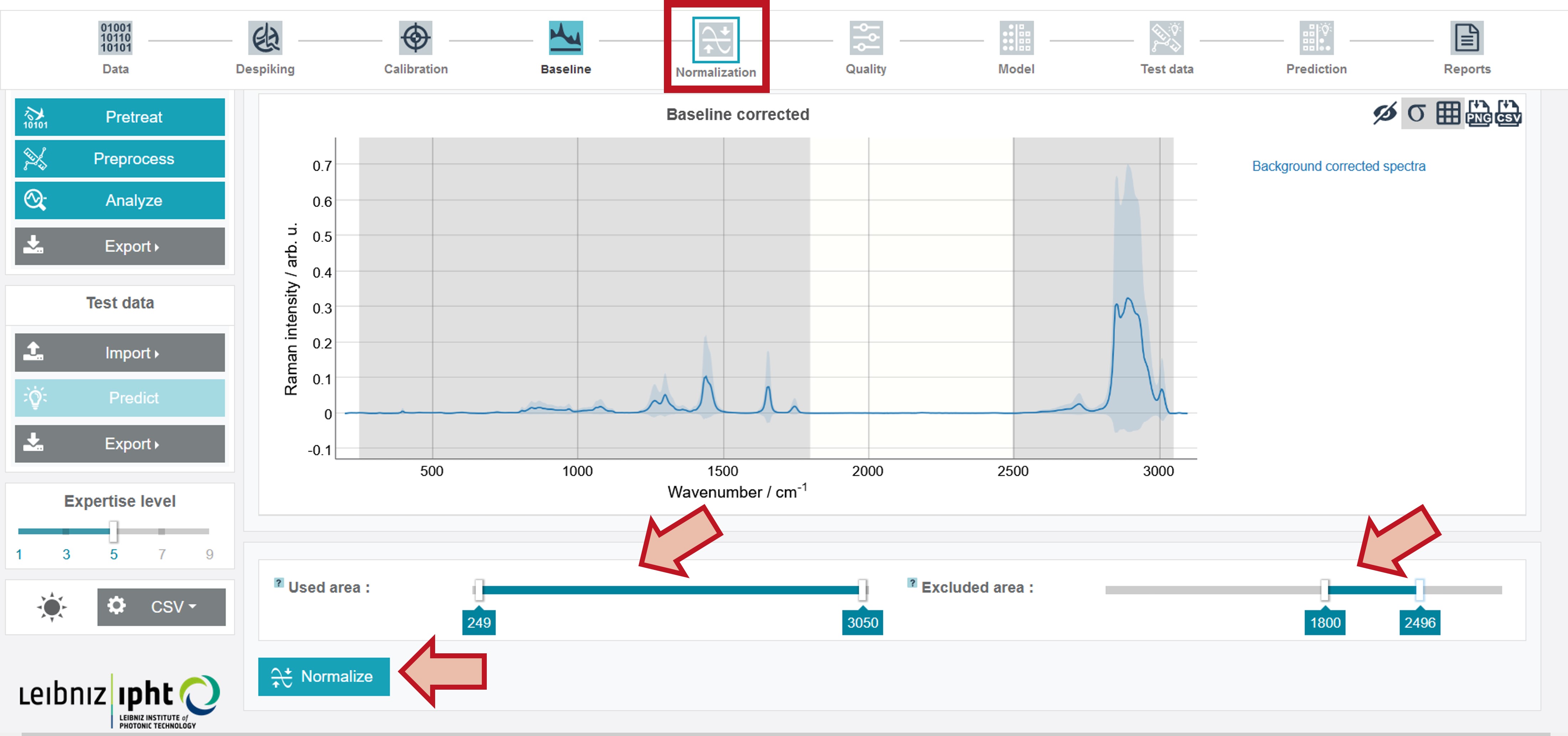
Preprocessing - Normalization
It is possible to carry out the normalization just for a defined spectral range. For this used and excluded areas can be set by sliding the cursors to the desired wavenumber (a fine-tuning is again possible with the arrow keys on the keyboard). For the oil training dataset set Used area from 249 to 3,050 and Excluded area from 1,800 to 2,496 and click * Normalize*.
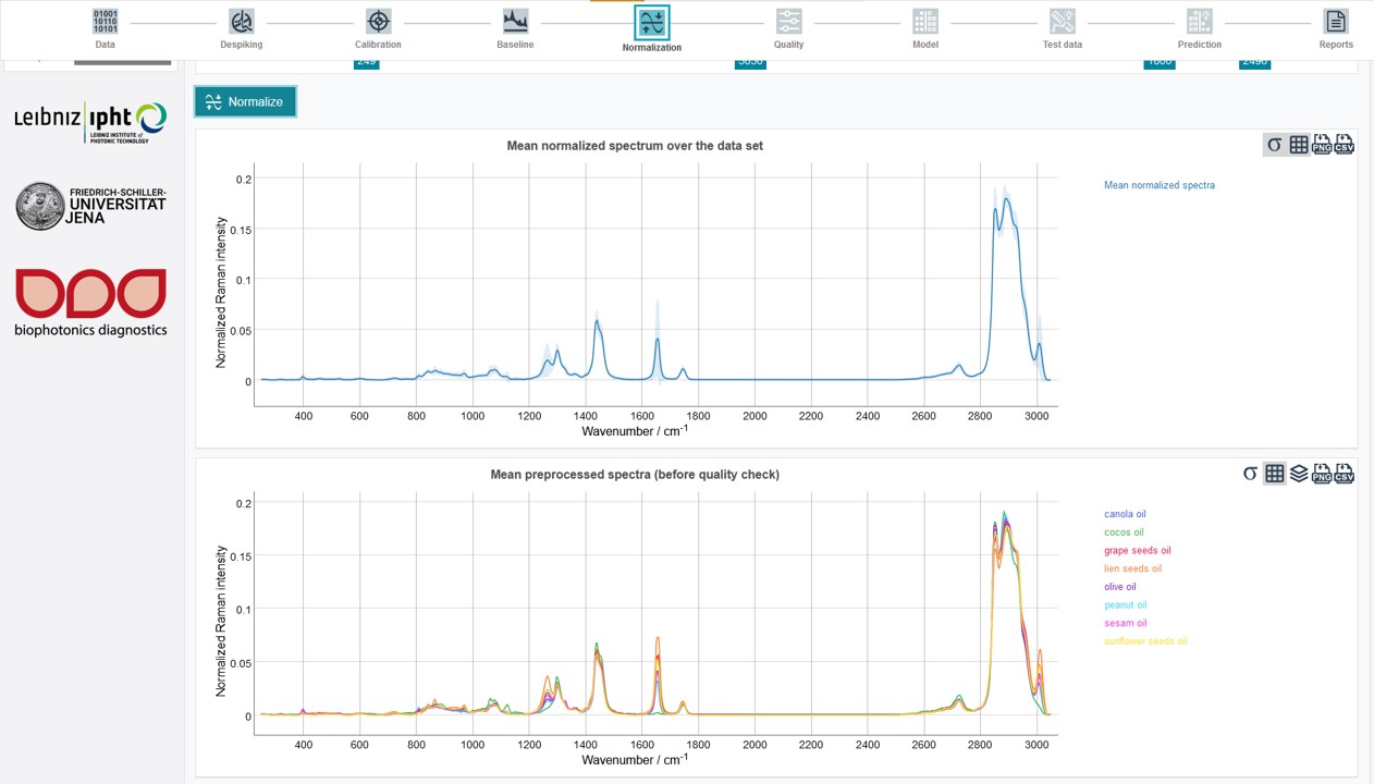
The results can be obtained as Mean normalized spectrum over the data set. In addition, the Mean preprocessed spectra (before quality check) (depicting the mean spectrum of every individual oil type) summarize the results of all pretreatment and preprocessing steps.
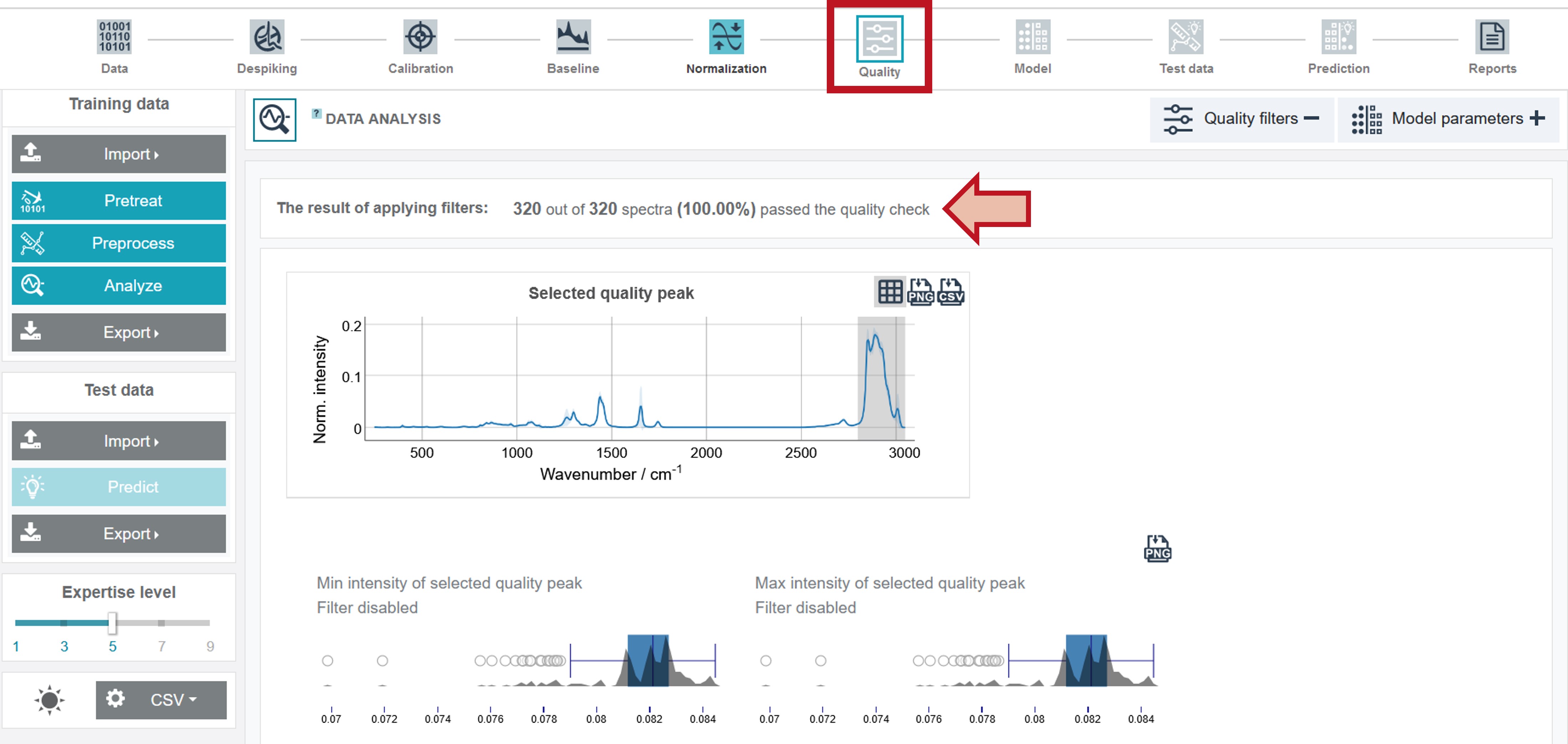
Quality filters
RAMANMETRIX offers various quality filters in order to sort out low-quality spectra that could diminish the precision of the model construction process. The quality filters can be chosen and adapted in Expertise Level 7 and higher. For this example, no quality filters were applied. Thus, all spectra included in the training dataset passed the quality check.
Modelling
RAMANMETRIX offers various methods that can be applied for the modelling process. Deeper information can be accessed again by the ? symbols.
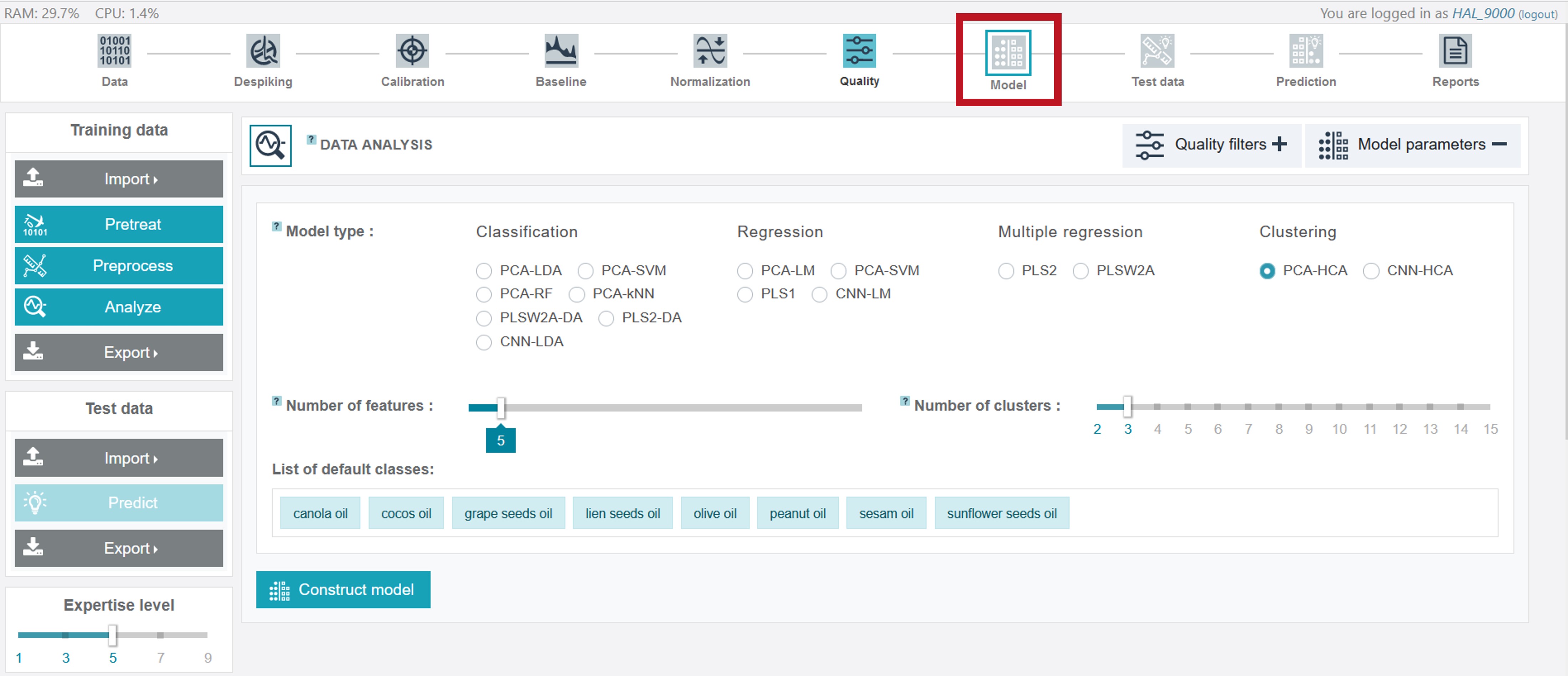
For the creation of an appropriate model for the oil training dataset the PCA-LDA classification model type was chosen, considering 9 features (the number can be adjusted by sliding the respective cursor) and the evaluation type 10-fold for the cross-validation.
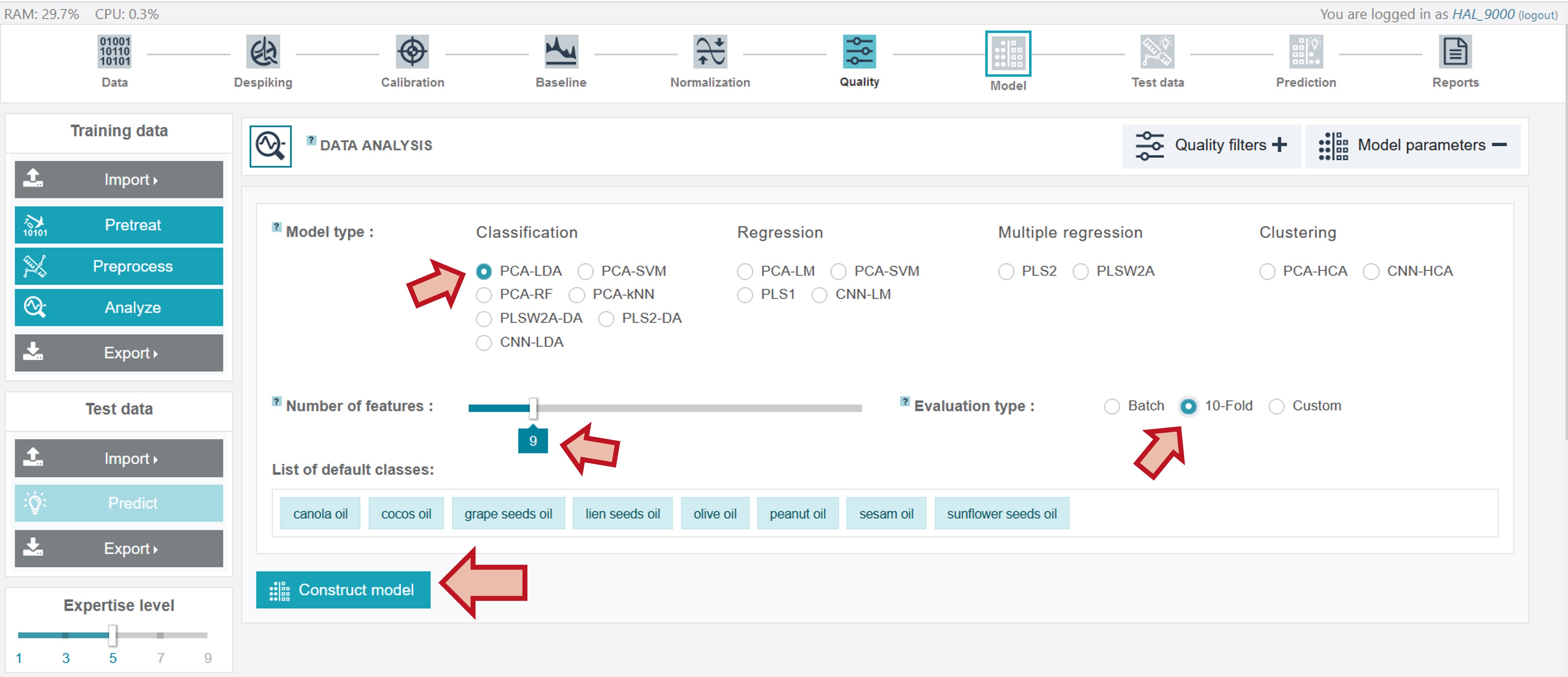
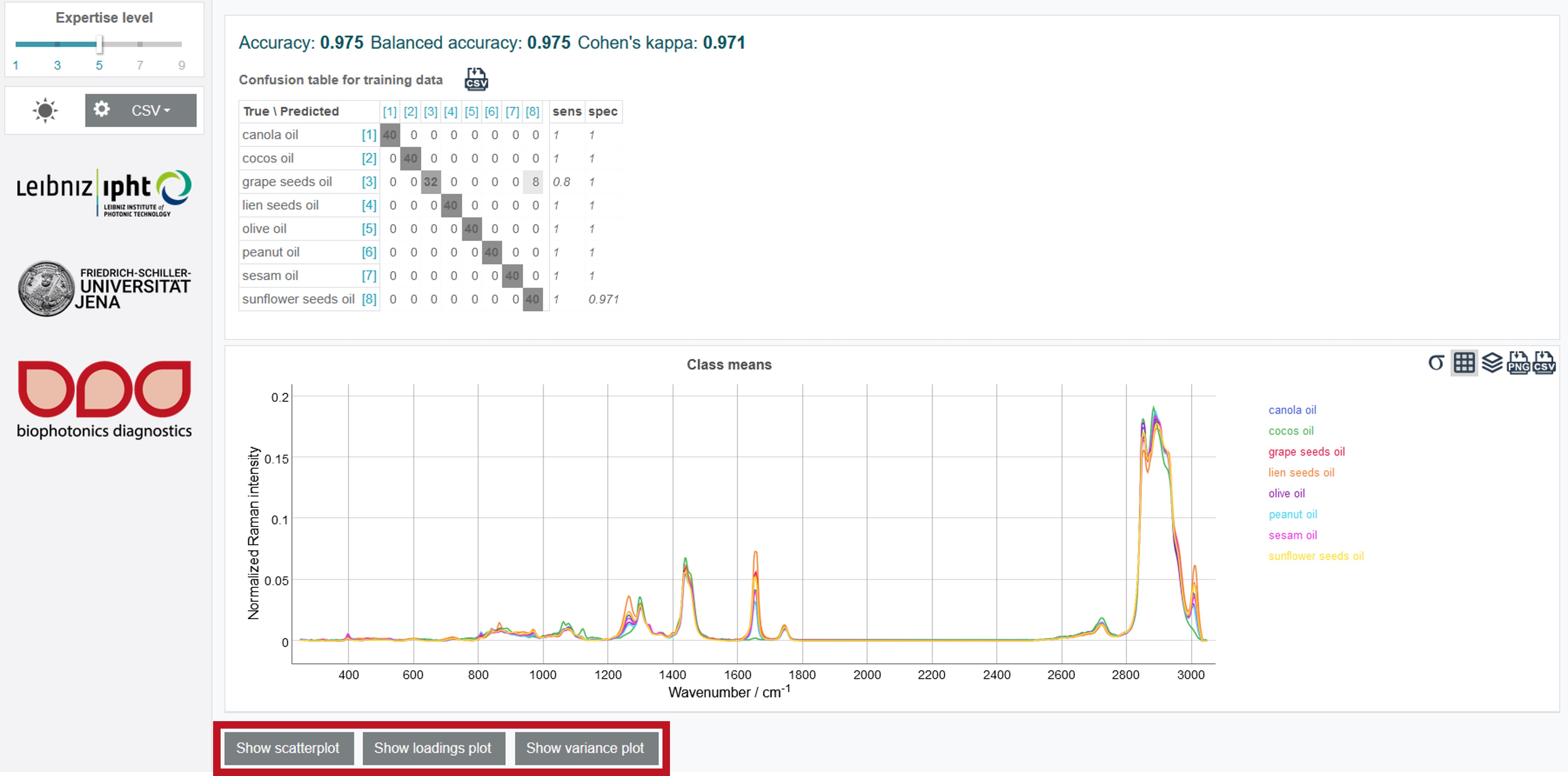
By clicking Construct model the results of the modelling process are presented in form of a confusion table with the respective accuracy value. The dark grey numbers show the number of correctly assigned oil types while the light grey mark the wrong assigned oil spectra. The sensitivity sens gives the ratio of the false negative results while the specificity spec gives the ratio of the false positive ones. In addition, the scatterplot, loading plot and variance plot can be shown by clicking on the buttons below the mean class spectra.
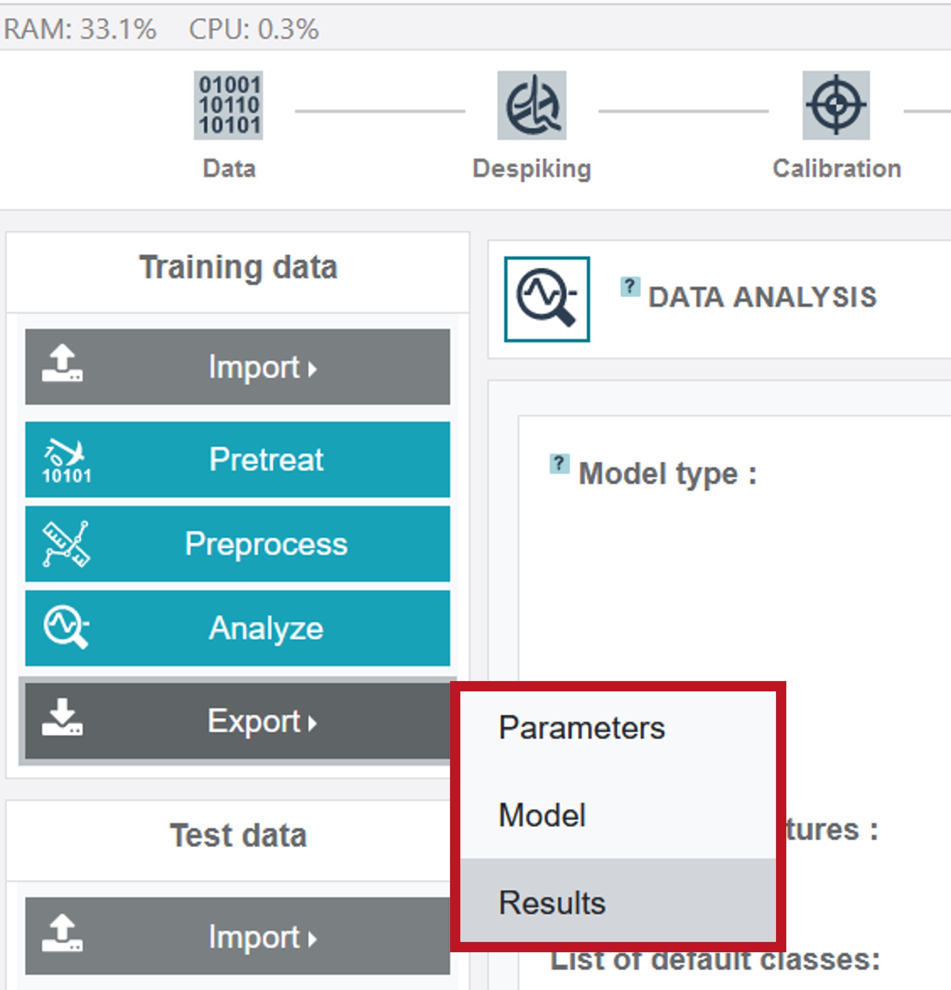
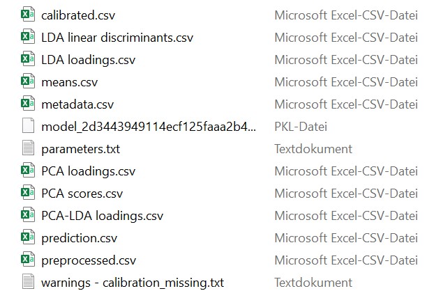
Parameters from the pretreatment and preprocessing steps, the created model (including the pretreatment and preprocessing parameters) and the results in form of a zip-file (including model, parameters and csv files of the plots) can be exported via the Export button at the left toolbar.
Testing the model
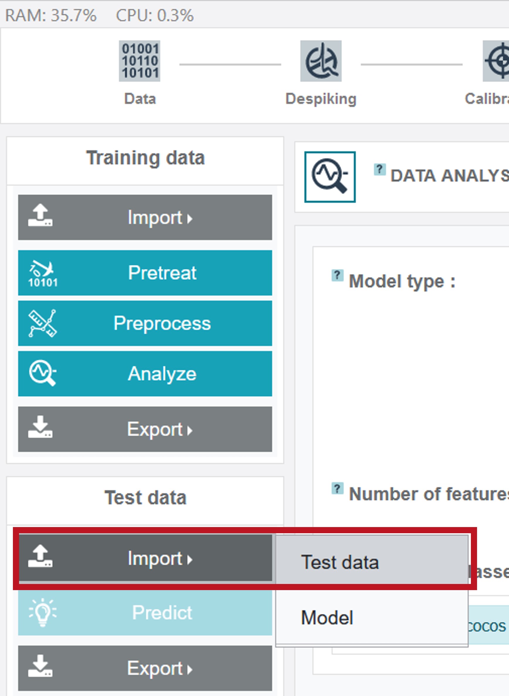
After creating the model it can directly be applied to a test dataset. The test dataset Test_Oil can be uploaded by clicking Import (Test data) on the left and choosing Test data.
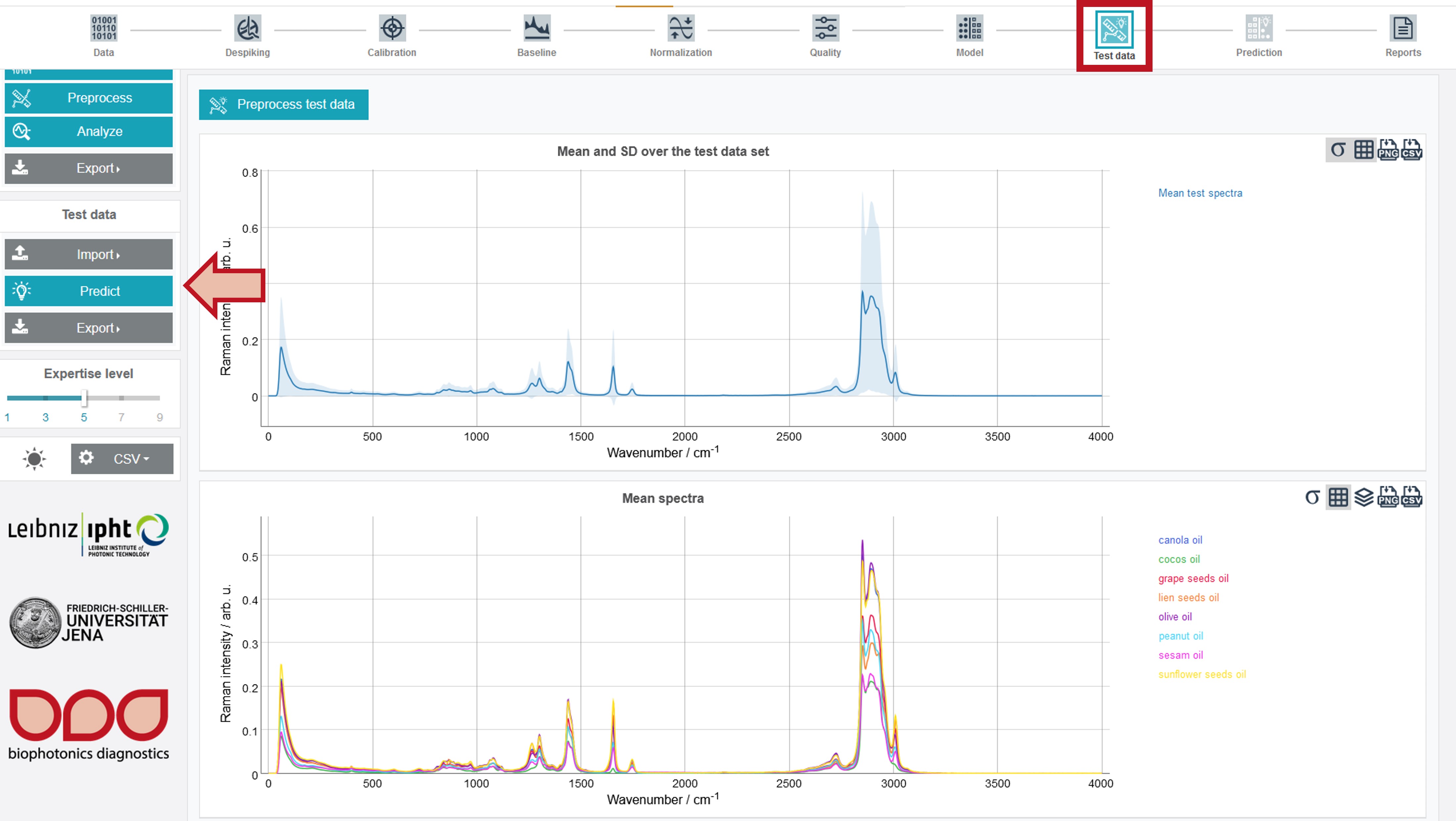
For the test dataset the Mean and SD over the test data set and Mean spectra for all oil types are depicted. In addition, the respective metadata can be accessed by clicking the Metadata button in the upper right, similar to the training data. The model can easily be applied to the test data by clicking Predict on the left toolbar.
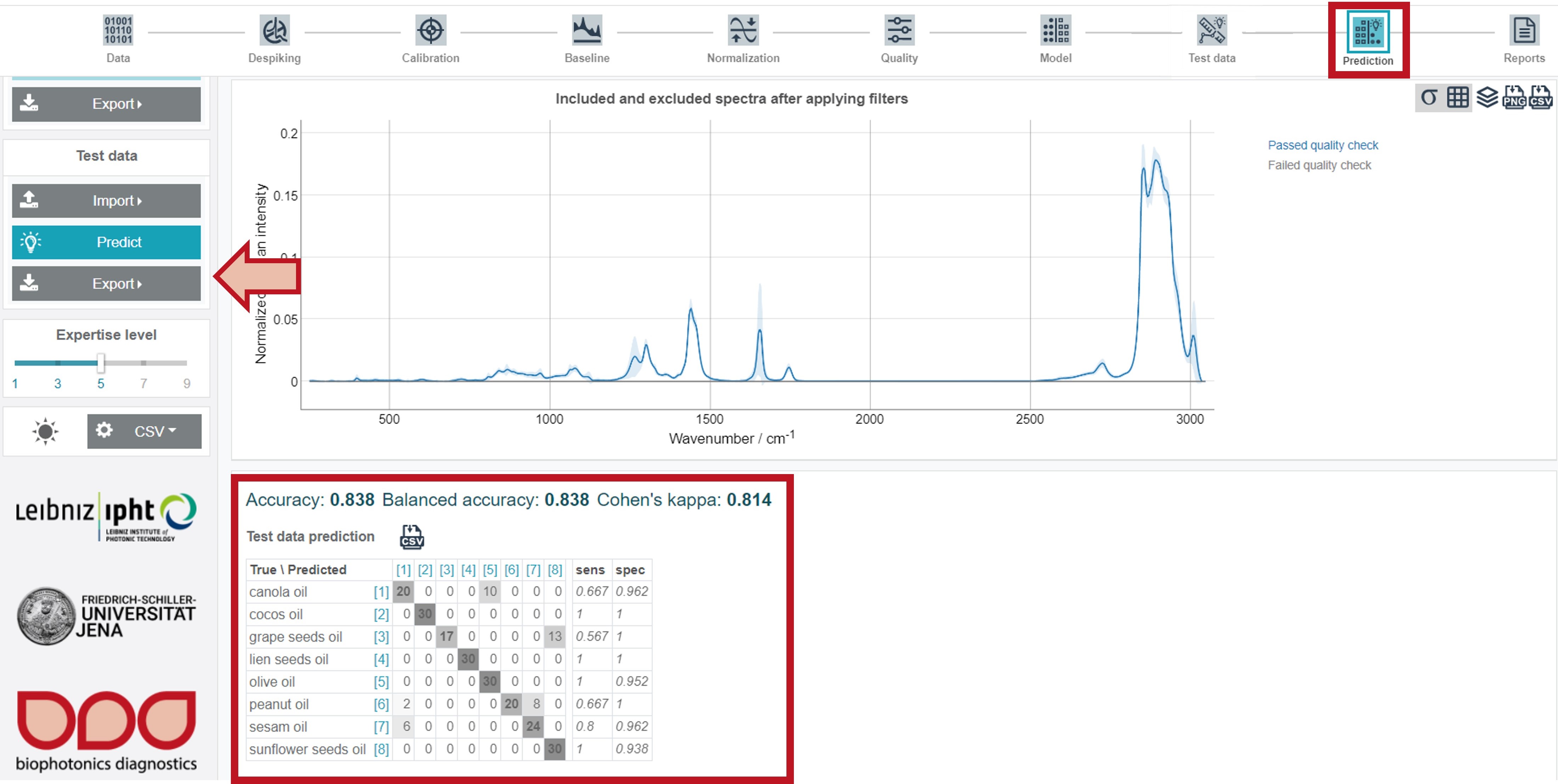
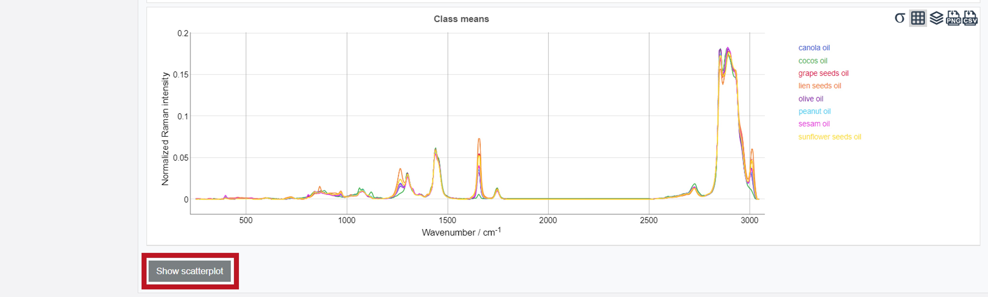
The results are presented, similar to the training data, in form of a confusion table. Additionally, the Included and excluded spectra after applying filters (depicting the pretreated and preprocessed mean spectrum over the whole dataset) and the Class mean spectra are shown. The scatterplots are available by clicking Show scatterplot. All test results can also be exported as zip-file via the Export button (Test data) on the left.
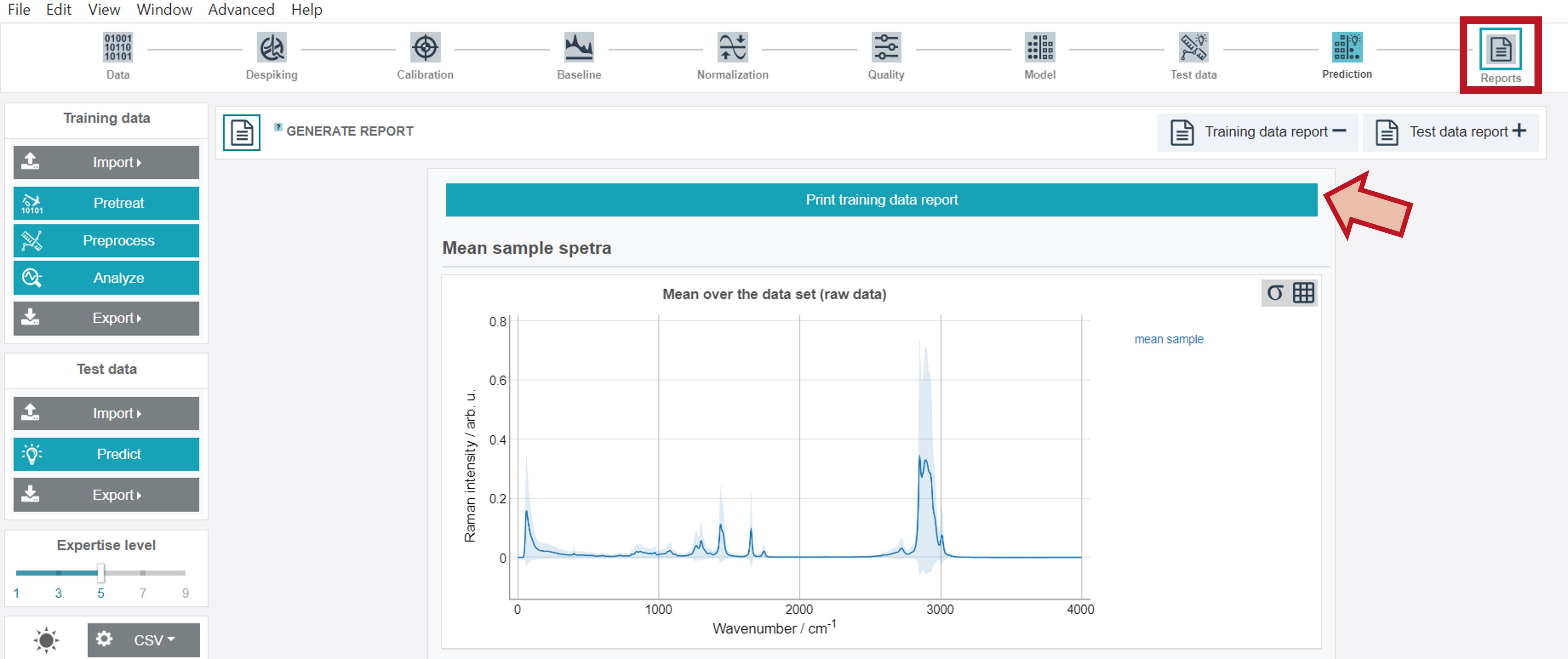
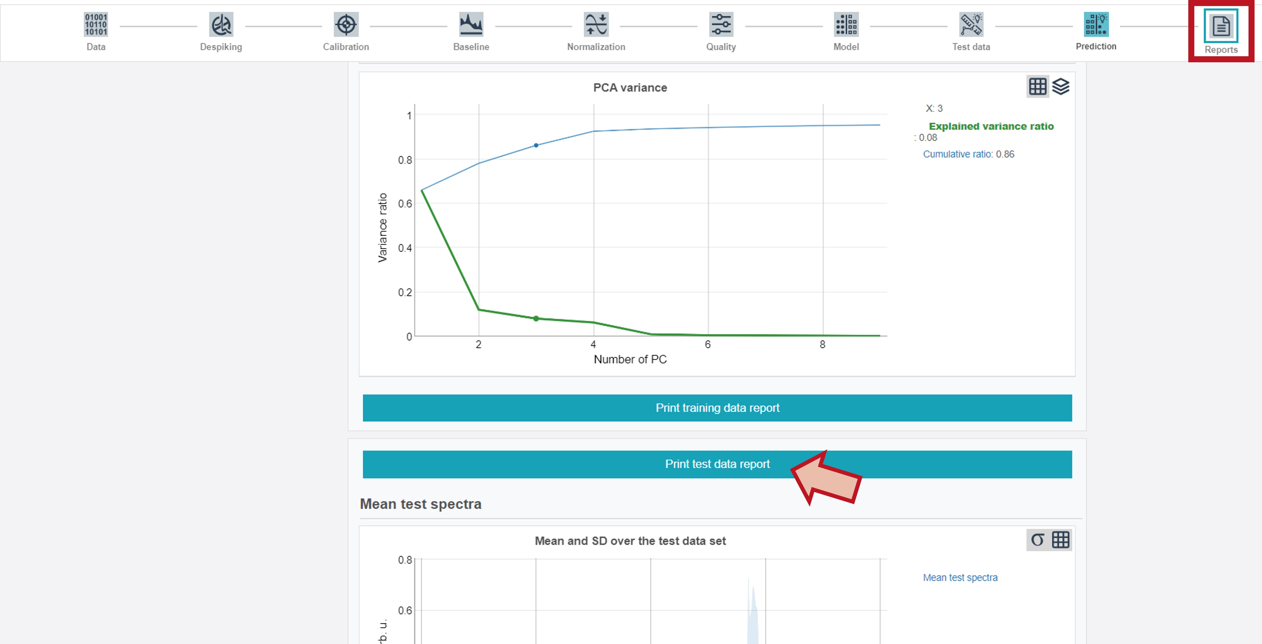
Training and test reports
Training and test data reports are additionally available via the right button (Reports) at the upper toolbar. By clicking Print training data report or Print test data report (button follows after the training report) all results can be either directly printed or saved as pdf-file.